An R Markdown Approach to Academic Workflow for the Social Sciences
- I'm not sure it could ever be this straightforward for academic research, certainly in the social sciences. And that's okay. We can still impose some order on our projects.
I’ve been thinking a lot about workflow lately because I’ve had some time and opportunity to do so post-tenure, but also because some co-authored projects have made me rethink what exactly I’m doing. I don’t think I have the worst workflow. Indeed, my research projects all go on my Github and I don’t do anything where a workflow based on mouse clicks could torpedo an entire European country. Still, my workflow is a bit messy if the reader were to peer underneath the hood of what I do. At least, I think it is. Heck, look at this from three years ago and wince at the horror of all that ugly-ass code cluttered in an R Markdown file. I’ve yearned to see if I can’t impose some more order on what I do in a way that’s just a little bit more obvious to me (and certainly more obvious to someone trying to replicate what I do). It’s also of interest to me as I desperately want to start training graduate students even if the opportunity may not necessarily be here at my current institution.
Emily Riederer’s post on R Markdown-driven development clued me into ways of rethinking how to make my R Markdown-oriented papers as R projects, even offering a nifty taxonomy of directories to include in an R Markdown project that can intuitively separate and classify the files in it. What I offer here is largely inspired/derived from what she proposes there, but with some tweaks that either 1) make more sense to me or 2) better communicate to my intended audience (i.e. students/researchers in the social sciences, especially political science).
I start with a table of contents to guide the reader through this post. I begin with one assumption that motivates me here that I think is important to say it loud. I proceed with my interpretation of a good workflow, however clumsy I’m stating it. I next offer an R project to academic workflow with a proposed taxonomy of directories to include in an R project directory. This approach even includes a sample project I did and uploaded in full to my Github so that readers can follow along. The bulk of the post that follows from that describes how to structure an R Markdown file that’s ultimately (and perhaps cynically) being used as an operating system (of sorts) rather than a simple Markdown translator for R. I close with some final comments, including how to automate some discussion of the statistical models in the paper.
- An Academic (Social Scientific) Workflow Can’t Be That Simple (and That’s Fine!)
- The Basic Workflow, as Concept
- Starting Your Project (and an Example Project)
- Structuring the R Markdown File
- Final Comments/Tidbits
An Academic (Social Scientific) Workflow Can’t Be That Simple (and That’s Fine!)
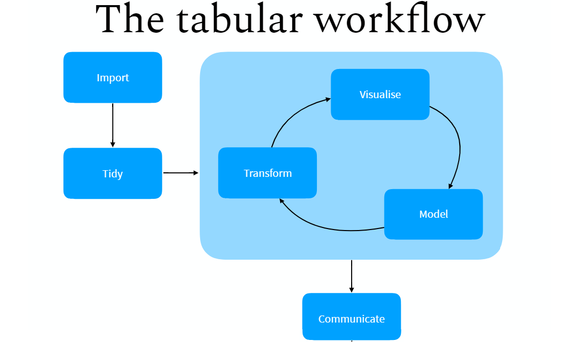
I’m a devout tidyvert, having converted to the tidyverse around 2013. I know “tidyvert” means something different in this context, but it’s the term I’ll use here since I practice my faith everyday. I remember looking with some kind of envy that my workflow couldn’t really converge on the neat diagrams that motivate the data science team working in the tidyverse. Therein, data are imported, cleaned/”tidied”, transformed/modeled/visualized, and then presented in a way that’s 100% reproducible and immediately understandable to a lay audience. I might be reading too much into such a minimal diagram and the maxims that I discern may not be as absolute as I suggest they are here, but it should be clear that a social science/academic workflow will invariably fall short of such a lofty ideal and a simple process for several reasons.
For one, an academic/social science project will often—perhaps almost always from my vantage point—rely on raw data that cannot be distributed in its current form as part of the project. In my various projects, I’ve used data from American National Election Studies, Correlates of War, European Values Survey, General Social Survey, and World Values Survey, among others. The raw data are not only not mine to distribute in its raw form, but the size of some of these files are prohibitively large to include. So, while the GML MID data might be 150 kilobytes, the six waves of World Value Survey data is about 1.6 gigabytes. It’s also not my data to distribute and so the type of project-driven development in R Markdown that Emily mentions on her blog isn’t 100% conducive to what we do. Our data directories in our projects can’t be read-only, sadly. However, that idea should still permeate the workflow.
Second, I think a lot of workflow guides in R Markdown miss that the academic project involves a lot of time on model-building, model-fitting, and staring at the results to see if they make sense. There’s a rinse and repeat, and a GOTO 10 at various steps along the way. We’re always throwing proverbial rocks at what we’re doing just to stress-test it and see if/when it breaks. There will never be a case—save the worst paper ever written to be desk-rejected with prejudice at every outlet—where a researcher gets a single data set, runs a model on it, and writes up the first results s/he sees. And yet, I think a lot of workflow tutorials don’t really communicate that. Certainly the tidyverse/data science diagrams mention a repeating process in the “explore” stage (see above), but the proposed workflow from that isn’t quite clear especially when the process sometimes involves returning to the drawing board and starting over again.
We basically code and do analyses until we feel confident with what we’ve done, and then we write up what we did and pray for an R&R or that the inevitable rejection takes just two months or fewer rather than six months. Your boilerplate workflow tutorial seems to imply everything is automated and there’s not a whole lot of prose that goes into the report that’s written. Again, I might be reading too much into these workflow tutorials but it’s how I discern them.
Still, I think the type of workflow I propose next (and will likely amend/tweak at various steps along the way) does well to approximate that while providing some flexibility for an academic project that is ultimately assembled in pieces. I’ll start with the overall framework as a concept.
The Basic Workflow, as Concept
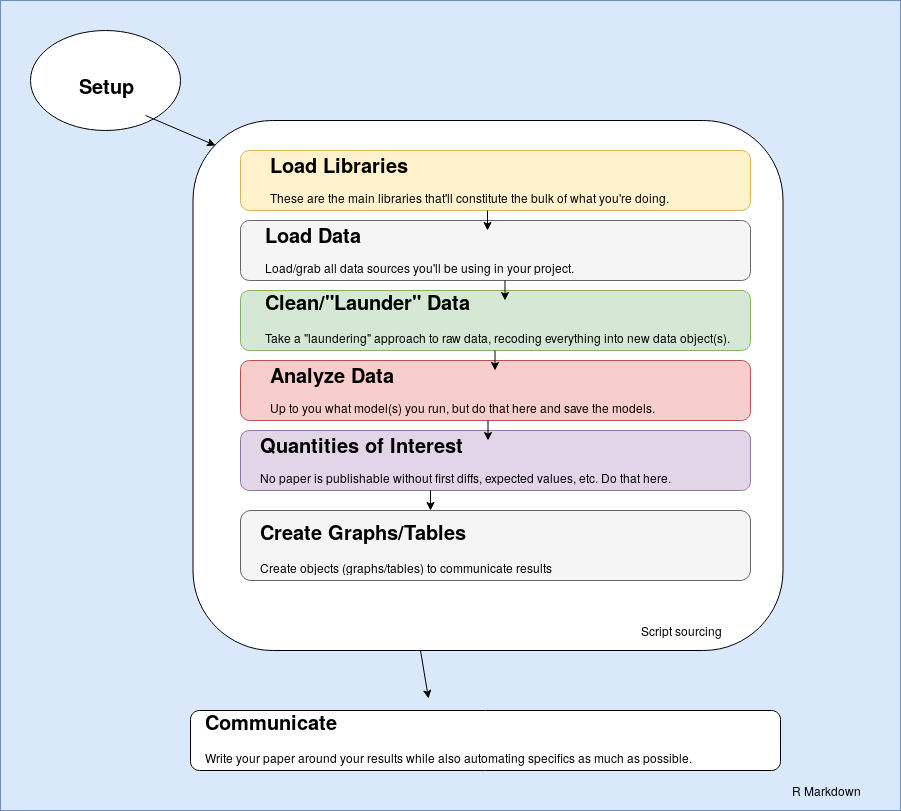
- The basic idea for an R Markdown workflow. Note: graph is hella ugly.
I don’t think anyone can describe workflow without a graph of some kind, so here’s my (clumsily created) interpretation of what I have in mind.
Basically, everything occurs within R Markdown and, depending on the size of the objects with which you’re working, may lean on R Markdown’s ability to cache chunks so you don’t have to always do everything from scratch. This does have one limitation that Emily explained to me via an e-mail, and it’s certainly an issue that those who advocate make-like declarative workflows will reiterate loudly. This treats R Markdown as something akin to an operating system when it was never intended for that use. R Markdown is instead a simple markdown translator. However, I think this is fine if you’re just working by yourself and aren’t as concerned with version control.1 Further, the analyses must ultimately be communicated as a document/report, which kind of implies that R Markdown should be a wrapper for whatever it is a researcher is doing. Workflow should be automated and reproducible but, for social scientists, the workflow is happening and evolving during the writing process. It’s important to impose some order on it, but also important to embrace it for what it is.
The process from there is straightforward (I think). There’s a minimal setup that is ultimately optional, but I’ll provide an example of what I think is a good setup in R Markdown. Thereafter, the most important libraries are loaded first. Then, the raw data are loaded from somewhere outside the project directory and stored as objects in the R workspace. Then, the data are cleaned, or “laundered”, into new data objects that are saved since these transformed data must be shared for reproducibility.
The next two steps are important parts of the analysis. There’s first a statistical modeling component where the researcher analyzes some response variable as a linear function of some set of covariates (i.e. I’m going to assume people are mostly doing regression analyses here). There may be multiple models estimated here that can be ultimately combined into one model object (i.e. a list). Next, the researcher generates quantities of interest, a sine qua non feature of empirical analyses in the present since it is no longer sufficient to run a set of regressions, present the results, and call it a day. Here, the researcher has considerable flexibility on what to do here and I’ll provide an example of what exactly the researcher can do in this stage of the project.
Finally, the researcher prepares some graphs or table objects to present in the document. Thereafter, the researcher proceeds to the laborious process of actually writing the damn paper. I’ll provide an example of this below.
Starting Your Project (and an Example Project)
I will be illustrating this with a sample paper (mostly gibberish) that I uploaded to my Github that analyzes six waves of World Values Survey data on attitudes toward the justifiability of abortion in the United States. I’ve used these data before as it’s one of my favorite toy data sets that I created for my quantitative methods class. I’ve talked about it here as well. Briefly:
This data set probes attitudes toward the justifiability of an abortion, a question of long-running interest to “values” and “modernization” scholarship. It appears in the surveys the World Values Survey administered in 1982, 1990, 1995, 1999, 2006, and, most recently, 2011. The variable itself is coded from 1 to 10 with increasing values indicating a greater “justifiability” of abortion on this 1-10 numeric scale. I’ll offer two dependent variables below from this variable. The first will treat this 1-10 scale as interval and estimate a linear mixed effects model on it. This is problematic because the distribution of the data would not satisfy the assumptions of a continuous and normally distributed dependent variable, but I would not be the first person to do this and I’m ultimately trying to do something else with this exercise. The second will condense the variable to a binary measure where 1 indicates a response that abortion is at least somewhat justifiable. A zero will indicate a response that abortion is never justifiable.
I’ll keep the list of covariates simple. The models include the respondent’s age in years, whether the respondent is a woman, the ideology of the respondent on a 10-point scale (where increasing values indicate greater ideology to the political right), how satisfied the respondent is with her/his life on a 10-point scale, the child autonomy index (i.e. a five-point measure where increasing values indicate the respondent believes children should learn values of “determiniation/perseverance” and “independence” more than values of “obedience” and “religious faith”), and the importance of God in the respondent’s life on a 1-10 scale. The point here is not to be exhaustive of attitudes about abortion in the United States, but to provide something simple and intuitive for another purpose.
Create A Directory, A File, and Some Subdirectories
First, create a directory where you’ll host your project (e.g. wvs_usa_abortion in my case). Then create a blank document and drop the following into it.
Version: 1.0

RestoreWorkspace: Default
SaveWorkspace: Default
AlwaysSaveHistory: Default

EnableCodeIndexing: Yes
UseSpacesForTab: Yes
NumSpacesForTab: 2
Encoding: UTF-8

RnwWeave: Sweave
LaTeX: pdfLaTeX
Save the file as an .Rproj file (e.g. wvs_usa_abortion.Rproj, in my case). The real benefit of an R project is that a person won’t ever have to bother with setwd() in RStudio. Open the .Rproj file as a project when ready to work on it.
Next, think of the following approach to your subdirectories.
my_project_name
+-- _cache
+-- _dross
+-- abstract
+-- appendix
+-- cover-letter
+-- data
|   +-- data.rds
|   +-- models.rds
|   +-- sims.rds
+-- doc
+-- figs
+-- presentation
+-- readings
+-- src
|   +-- 1-load.R
|   +-- 2-clean.R
|   +-- 3-analysis.R
|   +-- 4-sims.R
|   +-- 5-create-tabs-figs.R
+-- my_project_name.Rproj
+-- my_project_name.Rmd
+-- .gitignore
+-- README.Rmd
These are a lot of subdirectories, and I might fudge some things, but here’s the idea for each:
_cache: R Markdown caches code and stores it as chunks. I’ve never encountered a case where I actually looked at these files, which is why I recommend using a leading underscore to indicate it as a system directory (of sorts) that will appear at the top of the directory but that you can mostly ignore._dross: Part of my workflow philosophy is acknowledging that some code or paragraphs I write won’t survive a final edit, or just don’t work for what I’m wanting them to do for a particular analysis. It’s why I recommend creating a directory for dross. It’s not a directory you’ll need to make public but sometimes it’s good to keep old code or paragraphs around if the researcher can find them and use them again for another project. However, I think having a leading underscore is useful here so as to not confuse this directory with something integral for the analysis or manuscript. I call it “dross” for a reason.2abstract: Journals almost always require separate cover pages for anonymous manuscripts. It’s almost always a separate upload as well. Create a directory for that here. The cool thing is that R Markdown documents that have those YAML preambles become interpretable data sets for R. It’s possible—conceivably even easy—to automatically generate a simple title page from the YAML of the main .Rmd file for this directory, even though I’ve yet to do it. I might do that soon.appendix: You will have to write an appendix for the several dozen robustness tests that reviewers will ask of you. It will be around 20 pages. It will basically be a project within a project. Go ahead and create a directory for it. You cannot avoid it. Further, Steve’s Law of the Appendix is the probability of a reviewer asking for a particular robustness test increases the more robustness tests you’ve already done and provided as an appendix to accompany a manuscript for peer review. If you’ve already done 20 pages of robustness tests, the probability of being asked to do another one is basically 1.cover-letter: (OPTIONAL) Some journals may ask for a cover letter for peer review. If I recall correctly, PLOS ONE requires this. You may wish to write one if you’d like to make an extra pitch to the editor or warn the editor about reviewers you may not want for your paper.data: a directory for all your data/model objects that you’re creating in your project. Examples will include, in my workflow proposal here, R serialized data frames for your main data, statistical models, and simulated quantities of interest.doc: I got this idea from Emily’s post. She recommends creating a directory for any documentation or set-up instructions you may wish to include. It’s a good thing to have around and I have my own use for it as well that I’ll describe later.figs: Any graph I generate goes in this directory.presentation: This is a separate directory for an R Markdown presentation that I might prepare for a conference describing this project. Since you can make this lean on the workflow for the main manuscript, your presentation .Rmd won’t be too comprehensive. It should instead incorporate stuff you already did and stored.readings: (OPTIONAL) Every project I undertake involves me finding and saving a lot of PDFs for articles/book chapters that I may not use again. I end up storing those here.src: Got this idea from Emily’s post. This is where all the main .R files should go. Basically, the workflow scans thesrcdirectory for scripts to create stuff to store in thedatadirectory. The five files that I list are just examples and you may find yourself creating additional ones.
The final few files there are the recently created .Rproj file, the matching .Rmd file that will serve as the primary engine for our workflow (see diagram above), a .gitignore file you may wish to include should you upload your files to Github, as well as a README for users to communicate anything eles you’d like.
Structuring the R Markdown File
The academic workflow I propose relies on R Markdown as a workflow manager—even a de facto operating system—for academic papers within an already created R project. It begins with a simple setup with YAML and an ultimately optional first chunk to dictate some defaults for the R Markdown output. It proceeds with a next “main” R chunk that starts with loading important libraries to be used throughout the project. The next chunk proceeds with a series of commands that source code to load data, clean data, analyze data, and extract quantities of interest from the data. Thereafter, the results are processed as a figure or table to be inserted at various stages in the paper.
A Simple Setup
Setting up the .Rmd file is fairly simple. First, there is the YAML. My proposed workflow here leans heavily on my R Markdown template for academic manuscripts. Please read more about it here. I’ll note that I’ve since added a few extra options to this template. For example, endnotes: yes will convert footnotes to endnotes and removetitleabstract: yes will remove the title page and abstract. These are changes I’ve added to meet various journal standards along the way. However, I don’t think this the appropriate forum to belabor R Markdown or YAML. I’m assuming some familiarity with it already. I think the aforementioned post is a good place to start.
The next part of the setup process could conceivably be optional if the researcher felt like skipping it altogether. However, I think the following chunk at the beginning of the document (after the YAML) is useful for a lot of things.
```{r setup, include=FALSE}
knitr::opts_chunk$set(cache=TRUE,
                      message=FALSE, warning=FALSE,
                      fig.path='figs/',
                      cache.path = '_cache/',
                      fig.process = function(x) {
                      x2 = sub('-\\d+([.][a-z]+)$', '\\1', x)
                      if (file.rename(x, x2)) x2 else x
                      })
```
The first set of options tells R Markdown to cache everything by default, which I think is appropriate for analyses of bigger data sets or those that involve more complicated models. They also tell R Markdown to suppress any unnecessary warnings or messages that some lines of code may want to spit into the console (and thus be knitted). The next two options specify the directories for the cache and the figures. Do note: a researcher can always have R Markdown create these directories in lieu of the researcher manually creating these directories. The final option (fig.process) takes a close eye to discern what it’s doing, but it will change how R Markdown names figures. By default, R Markdown will name a figure as whatever the name of the chunk is and add a number to it. This command will strip the file name of the number, leaving a file named something like plot_sims.pdf instead of plot_sims-1.pdf.
Load Libraries
Next, create a chunk and name it something like loadlibraries and make it the next chunk in the R Markdown document. Here’s an example from the accompanying R Markdown file on my Github.
```{r loadlibaries, include=FALSE}
library(tidyverse)
library(stevemisc)
library(RCurl)
library(lme4)
library(dotwhisker)
library(broom)
library(modelr)
library(digest)
```
The libraries loaded here are at the discretion of the researcher. I’m still tweaking how I think about loading libraries and when I load them (i.e. all at the beginning or piecemeal when I need them). I do offer the following advice, though. First, load the most important libraries first. tidyverse and my stevemisc package are always the first things I load. Then, structure the libraries loaded into the R Markdown document by a loose order. In this case, I know I’m using RCurl to read my data from Github (and it’s the only reason I’ll be using it). Next, I know I’m using lme4, dotwhisker, modelr, and broom for the analysis section. The digest package is important for the end of my code.
Further, avoid function clashes when at all possible and, if at all possible, avoid loading an entire library if there’s only one function needed from it. For example, my 4-sims.R file uses the awesome merTools package for model simulations, but merTools has a separate select() function that will clash with dplyr (which is loaded from tidyverse). I use dplyr::select() a lot for data cleaning in anything I do and I don’t want merTools clashing with it, let alone clash with it before I start loading and cleaning data. So, not only do I avoid loading merTools before I start cleaning/laundering the data, but I don’t even load merTools at all. Instead, I load the function I want from it—predictInterval()—as merTools::predictInterval(). It’s the only function I need from that package, so there is no point loading the entire package if I can avoid doing so without too much inconvenience to myself. Basically, my workflow puts tidyverse above every other R package in importance.
Structure the Sourcing Chunk
The next R Markdown chunk will be doing the bulk of the analyses. Create an empty chunk as follows.
```{r source, include=FALSE}

```
Then, drop the following bits of R code in it and feel free to adjust to workflow preferences.
if (file.exists("data/data.rds")) {
  Data <- readRDS("data/data.rds")
} else {
  source("src/1-load.R")
  source("src/2-clean.R")
}

if (file.exists("data/models.rds")) {
  Models <- readRDS("data/models.rds")
} else {
  source("src/3-analysis.R")
}

if (file.exists("data/sims.rds")) {
  Sims <- readRDS("data/sims.rds")
} else {
  source("src/4-sims.R")
}
The intuition here is simple and consistent with a flexible workflow that both acknowledges that the academic workflow is not a simple process but also permits some fast-forwarding in the R Markdown compilation. For the data, model, and quantities-of-interest objects, the source chunk first checks if the object exists in the data directory. If it does, it loads it into the workspace. If the object does not exist, it sources the script(s) to create it (and, in the process, loads the object into the workspace).
I think this is an acceptable tradeoff especially for larger and more complex analyses, but it’s worth mentioning a few things that are imperative for the researcher. First, the end of the relevant script should be saving the object in question to an R serialized data frame in the data directory. Second, while it’s flexible to allow the researcher to adjust and tweak things like the main data frame or the statistical model(s), the researcher has to remember to ultimately save/commit those changes to the data directory. Third, the important limitation of this approach is the R Markdown chunk doesn’t scan the sourced .R files for changes. It simply scans itself for changes and, if it observes a change, re-runs the chunk. Again, this makes it more imperative for the researcher to know what s/he has done and committed within the sourced .R files and data directories, but it allows for greater speed in compiling the report without retracing too many steps.
Further, the researcher can just omit the if-else file.exists commands and straight source the scripts because they’ll be cached all the same when the document is compiled. However, I like this approach for a simple reason. Acknowledging the academic workflow process is not simple or linear, it nevertheless allows the researcher to skip ahead a few steps if appropriate. For example, assume I’ve already cleaned the data and estimated the model(s) I want. However, I need to write the simulation script now. I can load the data object and the model object within the R Markdown document rather simply instead of opening all those .R files in the src directory to run them individually. Further, loading R serialized data frames will invariably be faster than sourcing the scripts that create those files.
Loading the Data
Next step in the workflow is to load the raw data. I echo Emily’s advice that the raw data should be “read-only.” It’s why I have a massive data directory on my Dropbox that’s 270 gigabytes of raw data I’ve accumulated over the years. However, it’s not often the case a social scientist can share raw data. S/he can only share a finished data output. Nevertheless, the principle remains the same. Load the data into an object to later be cleaned/”tidied” and saved as a different data object.
For simple projects, like the accompanying project I uploaded to Github, there won’t be much in either the 1-load.R file or the 2-clean.R file. However, more realistic research projects will often rely on lots of different data inputs and have more complicated code for cleaning/laundering everything into a finished data object. It still makes sense to separate the files.
Cleaning/Laundering the Data
The next step in the research workflow is to clean the data. Here is the example 2-clean.R script I provide with the simple R project to accompany this post.
# note: carr and r2sd are copies of car::recode() and arm::rescale() respectively.
# I created these functions in my stevemisc package to avoid function clashes with those package and tidyverse packages.
WVS_USA_Abortion %>%
  mutate(ajd = carr(aj, "1=0; 2:10=1"),
         z_age = r2sd(age),
         z_ideo = r2sd(ideology),
         z_satisf = r2sd(satisfinancial),
         z_cai = r2sd(cai),
         z_god = r2sd(godimportant)) -> Data

saveRDS(Data, "data/data.rds")
There is not a lot to see in this simple exercise. In fact, most of the “raw” data were actually pre-processed prior to this project. However, I want to use it to emphasize four things.
First, always save the finished data object as a different data object. Notice I loaded the “raw” data as WVS_USA_Abortion and stored the cleaned version as simply Data. Call it whatever you like. I like Data because, in my mind after all these years, there’s no confusing 1) what that is (i.e. it’s the main data object) and 2) that the capital letter to start the name of the object tells me, in my head, that it’s a data object and not a vector or some other object. I’ve been using that shorthand for years; I think I got it from a Google style guide for R when I was in graduate school and stuck with it.
Second, rescale any independent variable that’s not binary and preferably rescale it by two standard deviations. There are two reasons for this. First, more complicated models—like the mixed effects models I use in this analysis—need a naturally occurring zero or it will whine in the console output. The model might not even converge. Second, there are so many cool practical reasons for scaling by two standard deviations, in particular. In this case, I am an unabashed disciple of Gelman and will recite the benefits of doing this as if they were scripture verses.
Third, never overwrite original columns. Create new ones instead. Last thing a researcher would want when dealing with all six waves of World Values Survey, for example, is to screw up coding a variable and overwrite the raw column in the process. Reloading that data might be a few minutes just to start over.
Fourth, make the final data object include only the important variables for replication of the main analyses as well as any additional analyses that become robustness tests in the appendix. That may not be evident in this simple example but, assume you’re working with the longitudinal General Social Survey as I recently did for my paper on the distribution of attitudes toward gun control in the United States. That raw data set has around 64,000 rows and over 6,000 columns. The corresponding data frame would be 1) huge and 2) include so much irrelevant stuff that it’d be an impermissible distribution of the raw data that interested users should be getting from NORC at the University of Chicago anyway.
Analyzing the Data
The next step in the workflow is to run the statistical models that constitute the main “results” section. Here, I assume the researcher is interested in some form of regression analysis and my simple example will be two mixed effects models on the justifiability of abortion, estimated as both a linear mixed effects model (on the 10-point scale) and a logistic mixed effects model (on the recoded variable).3
M1 <- lmer(aj ~ z_age + female +
             z_ideo + z_satisf + z_cai + z_god + (1 | year), data = Data,
           control=lmerControl(optimizer="bobyqa",
                               optCtrl=list(maxfun=2e5)))

M2 <- glmer(ajd ~ z_age + female +
              z_ideo + z_satisf + z_cai + z_god +
              (1 | year),
            data = Data, family=binomial(link="logit"),
            control=glmerControl(optimizer="bobyqa",
                                 optCtrl=list(maxfun=2e5)))

list("linear" = M1,
     "logistic" = M2) -> Models


saveRDS(Models, "data/models.rds")
It’s obviously imperative for the researcher to populate this R script as s/he sees fit, contingent on the exact research question. Thus, there is not a lot here that is worth belaboring. However, I will mention one thing. Consider storing/saving the model outputs as a list rather than individually save each model output as separate R serialized data frames or loading them as an R data file (.rda). Lists are flexible and can store objects of different types that can be loaded as an R serialized data frame.
Further, a researcher like me can become so flexible with lists and the lapply() function that s/he can estimate models and store them as lists simultaneously. Here is an example from a working paper that looks at how much we can explain attitudes toward decreasing immigration levels in the U.S. as a function of “economic anxiety” indicators like state-level unemployment differences at 1) a one-month interval, 2) three-month interval, 3) six-month interval, and 4) 12-month interval.
sunemp_vars = c("z_sunempr", "z_sunempr3md", "z_sunempr6md", "z_sunempr12md")


smodels = lapply(setNames(sunemp_vars, sunemp_vars), function(var) {
  form = paste("immigrld ~ z_age + female + collegeed + unemployed +
               z_incomeperc + z_lcindex + z_pid + wny + wpy + z_ec +", var, "*wpy +
(1 | survyr) + (1 | state) + (1 | state:survyr)")
  glmer(form, data=subset(AD, white == 1), family=binomial(link = "logit"),
        control=glmerControl(optimizer="bobyqa",
                             optCtrl=list(maxfun=2e5)))
})
The benefit of this approach is there is just one function to estimate and store four models. This is one “tidy” principle that’s worth sharing here (even as I struggle to find the source for this principle). If there is an identical or nearly identical code that the researcher is having to copy/paste at least three times in an analysis, consider making it a function instead. Lists are great complements to writing model estimations as functions and functions are great ways to avoid silly errors from copying and pasting the same line of code only to fudge some minor details (like one covariate in the example above).
Create Quantities of Interest
The researcher must next create some quantities of interest. 20 years ago, this step would’ve been completely optional despite great examples of quantities of interest existing from the early 1990s and King, Tomz, and Wittenberg telling us we should’ve been doing this already in 2000. It took about 10 years for it to become standard practice, but it’s definitely standard practice now. Researchers need to do more in the analysis beyond saying some independent variable of interest has a hypothesized effect that the parameters from the regression model suggest is likely discernible from zero.
There are great functions for this. Bayesian researchers already know about tidybayes, which has a suite of functions for generating quantities of interests as summaries of posterior draws. The ones I use the most are arm::sim() or merTools::predictInterval() for mixed effects models. The get_sims() function I wrote for my stevemisc package leans on arm::sim(). The example I provide here uses merTools::predictInterval() because the models are mixed effects models and this function (which itself leans a bit on arm::sim() too if I recall correctly) can also provide some simulations at varying levels of the random effect. This can be incredibly useful.
Let’s assume, for this exercise, that I’m interested in the effect of the importance of God in a respondent’s life on attitudes toward the justifiability of abortion. I want to simulate what is the expected value the respondent places on the justifiability of abortion (on both the 10-point and condensed binary scale) at each value of the importance of God in the respondent’s life.
First, I would use the data_grid() function in modelr to create a hypothetical set of observations in the 4-sims.R script.
data_grid(Data,
          .model=Models[[1]],
          ajd = 0, aj = 0,
          nesting(z_god)) %>%
  na.omit %>%
  mutate_at(vars(contains("z_"), -z_god), list(~replace(., . != 0, 0))) %>%
  mutate(year = 0) -> Newdat
Notice three things. First, we only need to create one fundamentally throwaway data object here, so we only need to extract the model parameters from the first model in our Models list since all variables are identical except for the different dependent variables. However, we need to create columns for both dependent variables (aj, ajd). Two, the nesting() function expands the data set by each value of z_god (itself a rescaled vector of the original godimportant variable). Third, the data_grid() function, by default, creates values that coincide with the mean (for numeric variables) or median (for binary variables). The follow-up mutate_at() function in the pipe recodes anything that’s not binary (i.e. has that z_ prefix) to be zero (i.e. the hypothetical mean before missing data). Finally, mutate(year = 0) will tell the merTools::predictInterval() function that we’re not interested in estimating the expected value of y by a particular level of the random effect. We just want the fixed coefficients and the observation-level error. The researcher can always omit this if s/he want the estimated value of y by different levels of the random effect. In a lot of applications, that might even be cool to see. Changing nesting(z_god) to nesting(z_god,year) and omitting mutate(year = 0) will create a new data set to simulate the variation by different years.
The next few commands will create summary simulations and extract simulations for both the linear model (i.e. M1, Models[[1]]) and the logistic models (i.e. M2, Models[[2]]), and save them as a Sims object to be saved as an R serialized data frame.
merTools::predictInterval(Models[[1]],
                          newdata=Newdat,
                          include.resid.var=F,
                          n.sims=1000, seed=8675309,
                          returnSims = TRUE) -> M1_summarysims

attributes(M1_summarysims)$sim.results %>%
  data.frame() %>% tbl_df() %>%
  bind_cols(.,Newdat) %>%
  mutate(godimportant = seq(1, 10)) %>%
  select(godimportant, everything()) %>%
  group_by(godimportant) %>%
  gather(sim, value, X1:X1000) %>%
  mutate(model = names(Models)[1]) -> M1sims


merTools::predictInterval(Models[[2]],
                          newdata=Newdat,
                          include.resid.var=F,
                          n.sims=1000, seed=8675309,
                          type = "probability",
                          returnSims = TRUE) -> M2_summarysims


attributes(M2_summarysims)$sim.results %>%
  data.frame() %>% tbl_df() %>%
  bind_cols(.,Newdat) %>%
  mutate(godimportant = seq(1, 10)) %>%
  select(godimportant, everything()) %>%
  mutate_at(vars(contains("X")), boot::inv.logit) %>%
  group_by(godimportant) %>%
  gather(sim, value, X1:X1000) %>%
  mutate(model = names(Models)[2]) -> M2sims


Sims = bind_rows(M1sims, M2sims)

saveRDS(Sims, "data/sims.rds")
I want to point out two things here, knowing full well that this code works as is mostly for this simple exercise. First, when available, always set a reproducible seed for simulations. My go-to seed is 8675309 because I work under the assumption that there’s something else horribly wrong in what I’m doing if the simulation output depends on Tommy Tutone. Second, take care when you can to extract not just the simulation summaries but the raw simulations as well (see returnSims = TRUE above). In my case, I find myself using the raw simulations to create simulated first differences for all simulations in addition to expected values of the dependent variable. Getting the raw simulations allows for more flexibility in presentation, especially at an advanced level of pipe commands in the tidyverse.
Obviously, this step of the research process is open-ended and the researcher should tailor it to whatever s/he wants to accomplish. However, it’s necessary to do these kind of simulations to create these quantities of interest. Setting seeds for reproducibility and extracting raw simulations from summaries of those simulations are good foundation approaches, though.
Create Tables/Figures
Next, the researcher should think about how s/he wants to present the results of the statistical model and the simulations. I do that as a separate chunk like this.
```{r createtabsfigs, include=FALSE}
source("src/5-create-tabs-figs.R")
```
For what it’s worth, I always like to render the graphs and create statistical tables every time I compile. The time it takes to execute the code is negligible so I don’t bother with the if-else approach I use for bigger objects like the data, the regression models, and the simulations.
The exact code here is to the discretion of the researcher. For example, this code will create a plot of the expected value of the justifiability of abortion at all levels of the importance of God to the repsondent, faceted by the type of model.
Sims %>%
  group_by(model, godimportant) %>%
  summarize(mean = mean(value),
            sd = sd(value),
            se = sd/sqrt(n()),
            lwr = quantile(value, .025),
            upr = quantile(value, .975)) %>%
  ggplot(.,aes(as.factor(godimportant), y=mean, ymin=lwr, ymax=upr)) +
  theme_steve_web() + geom_pointrange() +
  coord_flip() + facet_wrap(~model, scales="free_x") +
  labs(x = "The Importance of God to the Respondent (1-10)",
       y = "Expected Value (with 95% Intervals)") -> plot_sims
Here is what the plot_sims object will look like.
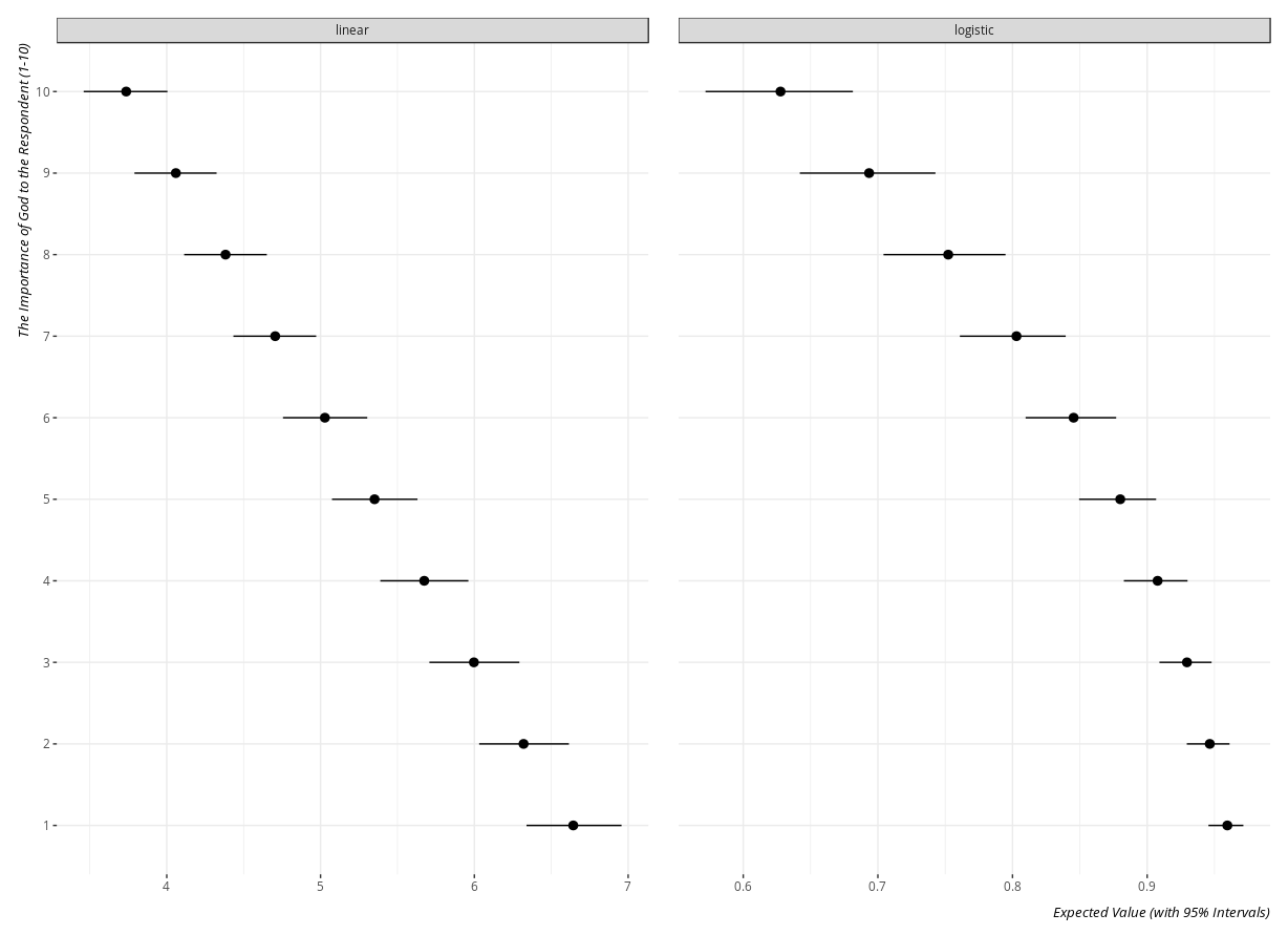
- Simulated Values of the Justifiability of Abortion by the Importance of God in the Respondent's Life
I do offer the following advice on whether a researcher should communicate results as a table or as a figure. Generally, the discipline is moving toward figures because figures are more aesthetically pleasing and more accessible to a lay audience. A researcher can reach more people with greater ease with a dot-whisker plot than s/he can with a regression table. Frederick Solt’s dotwhisker package is awesome for this and every R user should download it. I even use it in this simple exercise.
Do keep in mind, though, the following limitations of graphs in a scholarly journal. First, don’t create a graph that would lose any interpretatability if it were printed in black and white. Lean more on shapes than colors in dot-whisker plots for that reason. Second, I would caution against using dot-whisker plots to communicate the results of more than three (maybe four) statistical models for any individual graph. Take a look at Figures A.3 and A.4 in the appendix for “The Effect of Terrorism on Judicial Confidence”, a 2017 publication of mine in Political Research Quarterly. Here, I’m doing what looks like 16 different analyses summarized across two different figures wherein I say, basically, “if this looks unreadable it’s because that’s the point. Nothing is changing based on these different estimation procedures that reviewers are asking of me. Everything of interest is still discernible from a null hypothesis of no effect.” However, look what’s happening in those two figures. Both lean heavily on colors that could be lost in printing to black-and-white or may be lost on the colorblind and ggplot begins to exhaust immediately identifiable shapes after around three or four. There are space/”dodging” considerations here as well as the dots and whiskers come so close together these plots start to look more like caterpillar plots.
I would’ve made these tables instead and I chalk this approach to me being so young and impressionistic at—checks wallet for birth date—32. Oof. Here, I was just beginning to embrace the tables2graphs philosophy, but I was leaning too much into it. Learn from my mistakes. We’re always Gallant in the present to our younger Goofus as scholars.
Last Chunks for Reproducibility
Next, create the following chunk to follow the createtabsfigs chunk.
```{r reproducibility_stuff, include=FALSE}
# require(digest)
# plyr::ldply(mget(ls()), digest) # Meh, I like this way better below.
as.data.frame(do.call(rbind, lapply(mget(ls()), digest))) %>%
  rownames_to_column() %>%
  saveRDS(.,"data/md5s.rds")

devtools::session_info() %>%
    yaml::write_yaml("doc/sessioninfo.yaml")

sink("doc/sessioninfo.txt")
sessionInfo()
sink()

```
I got part of this idea from Emily’s post about creating a doc directory for supporting documentation for the R project. In this case, I’m dropping the current session info (i.e. the version of R, the packages I’m using, and the operating system) just in case a failure for another researcher to reproduce what I’m doing might be a function of different package versions or whatever else. I create two versions of the same file: a raw .txt file from a sink dump and a more sophisticated YAML document. Both have the same information even as the YAML file has some cool properties.
The code before it uses the digest package to create MD5 hashes for every object loaded into the data frame as a result of the analysis. Thus, a user interested in reproducibility (even future you for your own projects) can compare the MD5s s/he generates to the ones a researcher (i.e. me or you) provides for replication. I store this in the data directory because it’s an R serialized data frame.
Final Comments/Tidbits
The final step of the workflow process is to, well, write the damn paper (or at least finish writing it, assuming that the literature review and theoretical section are done prior to the analysis). Much of that is up to the interested reader to figure out for her/his individual project.
I do have the following pieces of advice. First, do the bare minimum R coding in the middle of the document. That should be done already and included in the top of the document. The choice is ultimately to the discretion of the individual researcher but the place in the document where the researcher should be writing about the results of the analysis should not be the exact same place where there is also code generating the results. It clutters the writing process (I think). So, it’s why I recommend doing the coding stuff first and just creating a simple chunk for a figure or table that will not interfere with the writing that the researcher will do around it.
```{r plot_models, fig.width=11, fig.height = 7, echo=F, fig.cap="Dot and Whisker Plots of the Two Models I Estimated that Are Totally Cool and Awesome"}
plot_models
```
I think this is as clutter-free as possible since I’m just calling an object (a plot) that I already created, which my setup already conditions to save in the figs directory as the chunk name (i.e. plot_models). However, I do recommend playing with the fig.width, fig.height and certainly the fig.cap properties here. Thus, there will always be some clutter when including a figure in an R Markdown document, but this approach minimizes it.
Second, automate the discussion of the statistical analyses as much as humanly possible. This is where I think R Markdown really shines as a framework for executing and summarizing statistical analyses. Notice, in the middle of my example document, I included the following paragraph.
The t-statistic associated with the importance of god coefficient is
r round(tidy(Models[[1]])[7,4], 3)in the linear model and the z-statistic for the same coefficient isr round(tidy(Models[[2]])[7,4], 3)in the logistic model. The precision of both statistics suggests an effect that we can comfortably discern from zero.
Assuming for the sake of illustration that this was an academic paper that was estimating the effect of religiosity (i.e. the importance of God in the respondent’s life) on attitudes about the justifiability of abortion, this code ganked a broom::tidy() summary of the model objects, identified (after already knowing where it would be) the associated t and z statistics and summarized them. Thus, the transcription error for discussing the statistical results is zero. That’s such an awesome feature of R Markdown. Further, these quantities can be generated and stored as standalone objects in a previous chunk if the researcher is uninterested in embedding as many R commands (i.e. round(), broom::tidy()) in a single line as I do here.
Feedback welcome and this post might be fudged as it is with additional tweaks that come to mind. I’m thinking about making this an R package as well.
-
I still haven’t figured out collaborative R Markdown projects since version control will clearly become a priority under those circumstances. Therein, I think there needs to be explicit delegation of tasks (i.e. one person only does the methods stuff) or use of version control software like git. ↩
-
I also call it “dross” because I remember being obsessed with this song as a senior in high school. Ah, youth truly is wasted on the young, to reference another lyric from that band. ↩
-
I probably wouldn’t estimate this DV as normal-continuous with a straight face for peer review, but, alas, you can start to get away with that when an ordinal variable has more than seven values. ↩
Disqus is great for comments/feedback but I had no idea it came with these gaudy ads.