How Should You Store/Load Your Bigger Data Sets? An Experiment With Six Waves of World Values Survey Data

- World Values Survey
How should you store and load your bigger data sets? Academics increasingly work with larger data sets but still mostly rely on computation through their personal computers. Cloud computing is available, either through Amazon or the university, but there’s a greater convenience in eschewing the cloud and analyzing the data on a personal computer. This is certainly how I approach things as I work in R, even after all these years.
However, there are costs with this approach that I’ve yet to address. Namely, a decent desktop and laptop (16 GB RAM each) still won’t save the user (i.e. me) from getting bogged in load times for the larger data sets. The World Values Survey in its longitudinal form—which I’ve used the most for my various research projects—is around 1.6 GB in disk space (contingent on the particular file, as I’ll discuss). It’s certainly not the largest data set any political scientist has ever used, but its 1,410 columns and 341,271 rows will be a fair bit larger than at least 90% of other data sets a political scientist will use at a given time. Should the need arise to run a few regressions on the data, a user will have to wait a few minutes for the data to load before spending any additional time recoding the data or running regressions.
I’ve wrestled with this for a while and have explored alternatives for how to save/store larger data sets and—more importantly for me—how to load them quickly. What followed is a quick experiment with the longitudinal World Values Survey (WVS) data on the quickest way to store/load data that could be plausibly construed as “big.”
The Setup
The setup for this experiment leans heavily on my approach to data workflow, in which I take a “laundering” approach that stores raw data in a data directory on my Dropbox. Thereafter, to facilitate reproducibility for a given project, I ‘launder’ the data fresh for each project but always leave the raw data untouched. Whereas I’ve worked with WVS data for the past 10 years, I have a standing wvs subfolder in my data directory on Dropbox and have stored various WVS formats there. For transparency’s sake, the last download I did of the six waves of WVS data came from its April 18, 2015 update.
Again, the data span 1,410 columns and 341,271 rows. This might not be the largest data set in wide use for political scientists, but it is among the biggest and would in all likelihood be the largest public opinion/attitudes data set that is widely available today.
I have saved the following formats of WVS data over the years. First, I have original downloads that WVS provides of its data as an R .Rdata file as well as an SPSS .sav file.1 In the past, I had loaded that WVS data and saved it as two different serialized data frames. The first is an R serialized data frame through the readRDS() function that comes standard in R. The second format is a fast serialization through the {fst} package.
The final format is an SQLite database. SQLite is one of many relational database management system options. I’m still teaching myself the ins and outs of various SQL standards, but SQLite’s main advantage for R users is its more lightweight nature. My (limited) understanding is SQLite is not ideal for when there are a lot of users making a lot of queries on a database at a given time. However, that limitation won’t apply to an individual R user trying to access a data source. This should make SQLite a go-to for relational database management sytems for users interested in doing their own statistical analyses and queries on larger data sets.
This amounts to five different versions of the same data source I have in my WVS subdirectory. For the sake of this experiment, I looped through a load of a particular format 10 times and saved the time it took to perform the task into a data frame. This is not the most elegant code, but here is what this loop would look like for the .Rdata format.
# load rdata method -----
# -----------------------
setwd("~/Dropbox/data/wvs")
library(tidyverse)

rdata_times = data.frame()

for(i in 1:10) {
  main_call <- system.time(load("WVS_Longitudinal_1981_2014_R_v2015_04_18.rdata"))
  times <- as.data.frame(t(data.matrix(main_call)))
  rdata_times = rbind(rdata_times, times)
  print(times)
}

rdata_times %>%
  mutate(Method = "load (Rdata)") -> rdata_times
The Results
Which Format Has the Fastest Load Time?
Here is a box-and-whisker plot of the load times across the 10 trials for each format. The results are pretty clear that the fastest load times came when the data were stored in some format other than what WVS provides for its users.
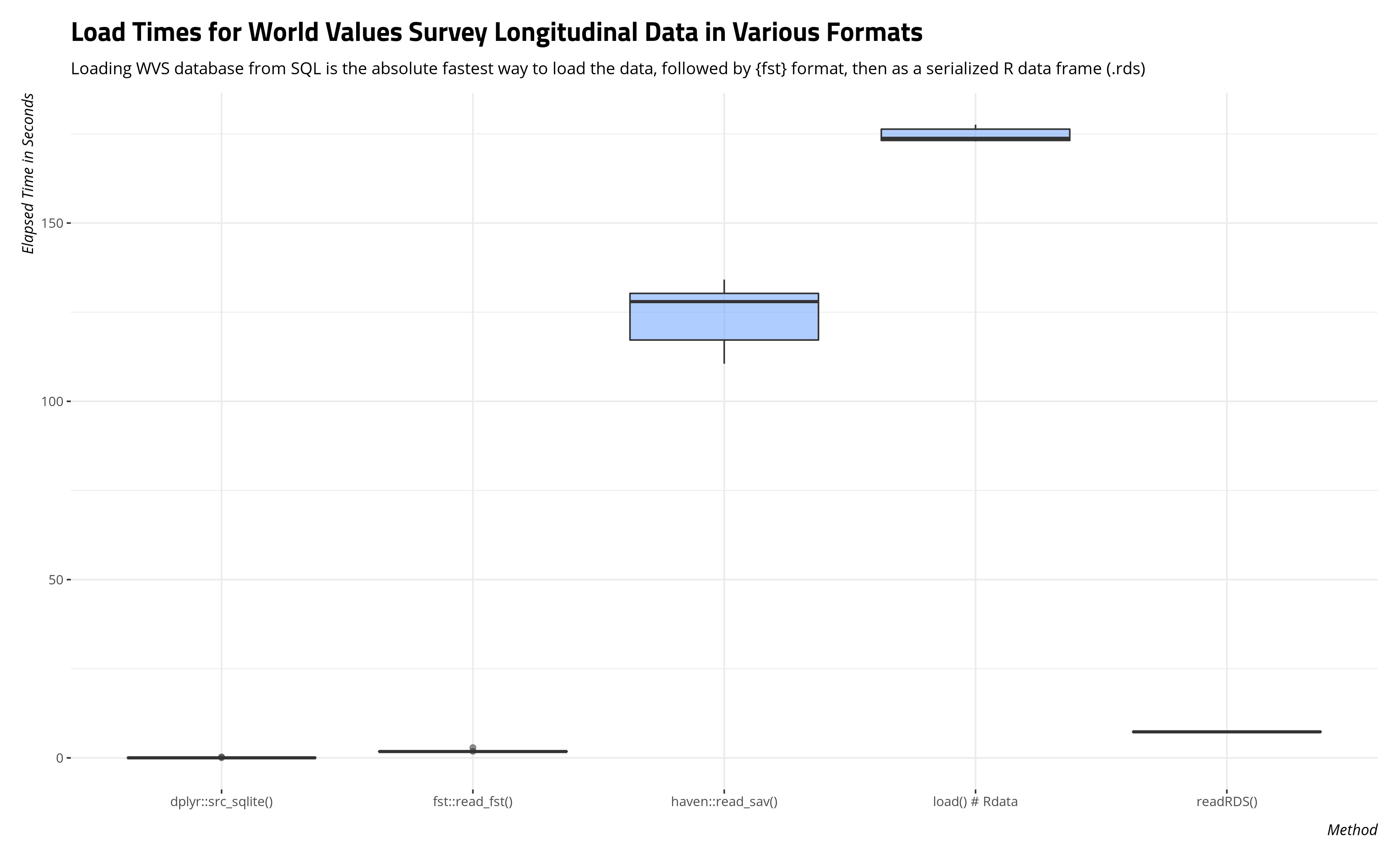
The box-and-whisker plot will easily communicate the scale of time saved through loading the data frame as an SQLite database or serialized data frame. The table below will summarize the average load time and standard deviation of a load time as well.
| Method | Mean Load Time (Seconds) | Standard Deviation Load Time (Seconds) |
|---|---|---|
| dplyr::src_sqlite() | 0.05 | 0.09 |
| fst::read_fst() | 1.90 | 0.34 |
| haven::read_sav() | 124.06 | 8.53 |
| load() # Rdata | 174.63 | 1.93 |
| readRDS() | 7.30 | 0.03 |
The average load time in R for an SQLite database of this size was .05 seconds, which is an almost instantaneous load time on par with calling in data(mtcars) in base R. The average speed of that load time is roughly 40 times faster than loading the data as a serialized data frame through the {fst} package and about 160 times faster than loading the data as an R serialized data frame.
The load times for the standard objects you can download on the WVS’ website stand out. All told, the typical load time for a standard WVS download as either an SPSS file or Rdata file is more than two minutes (SPSS) or almost three minutes (Rdata). That’s a lot of time spent waiting for the data to load into an R session. It may not seem like it, but the user will feel it when it’s happening.
Another Consideration: Object Size
This experiment would be incomplete without a consideration of the storage of these various data frames. A SQLite database (and presumably other SQL-standard relational database management systems) might have the fastest load times but are they the most economical means to storing data?
| Data Type | Disk Space (in MB) |
|---|---|
| SQLite | 307.47 |
| Rdata | NA |
| SPSS (sav) | 578.31 |
| Stata (dta) | 569.94 |
| Serialized Data Frame (fst) | NA |
| Serialized Data Frame (RDS) | 45.90 |
The answer here suggests a trade-off between load speed and disk storage. The SQLite database takes up the most disk space despite being the fastest to load. It’s a testament to how fast relational databases are that they load that quickly despite consuming that much disk space. However, a user interested in an optimal trade-off between size and speed may wonder if that approach is worth it when hard drive space may be an issue.
Elsewhere, standard binaries for R or statistical software users—like R’s Rdata format, SPSS’ .sav format, or Stata’s .dta format—consume a fair bit of disk space but offer little in the way of speed of access.2 This might make them a worst-case scenario, at least for R users. A R user who accesses the WVS data in SPSS’ native format has a file that takes about a third of the disk space but takes well over 2,000 times as long to load, on average.
There’s an intriguing trade-off between size and speed for the serialized data frames. The {fst} serialized data frame consumes only 182.24 MB of disk space but will load in just under two seconds, on average. That amounts to a binary that is more than three times as small as an SPSS binary but takes fractions of the time to load into an R session as the SPSS binary. The R serialized data frame is the smallest format of all options under consideration here, measuring at a bite-sized 45.89 MB. It does take a discernibly longer time to load relative to the {fst} format—about four times as long, on average. However, the compression is optimal and will hog far less space on a cloud storage or hard drive as some other options.
Conclusion
How should you store and load your bigger data sets? There’s value to learning how to save your data as an SQL-standard relational database. I chose SQLite but I doubt the central takeaway would differ if the database were MySQL or PostgreSQL. The load times for the relational database were discernibly faster than the other options.
However, the SQLite database consumed the most disk space by far. If hard drive space is a premium, the user may want to consider a serialized data frame approach. Data frame serialization through the {fst} package is the faster of the two options but the R serialized data frame (RDS) compensates for the relatively longer load times with better standard file compression. The R serialized data frame was the smallest of the files under consideration here and is about 1/4th the size of the {fst}-compressed data frame.
There are some tradeoffs worth belaboring. Consider that the relational database (SQLite) and the {fst}-compressed serialized data frame load the fastest and the {fst} option has the added benefit of great file compression on the hard drive. However, both approaches, at least as far as I know, discard variable labels in the data frame. I’m fine with this tradeoff because WVS data are well-sourced, both online and as downloadable PDFs. I have a lot of experience with variable names as well. However, users still learning the ropes of the WVS data may want those variable labels, especially if they’re proficient with the {sjmisc} package or like the get_var_info() function that I wrote into my stevemisc package. Thus, the user may want one of the binary formats (R, SPSS, or Stata).
In addition, there is still a startup cost here for the SQLite approach, the fst approach, and even the R serialized data frame approach. The user will still need to load the data as one of these binaries and then save/store the data as one of these other formats. Ideally, this is just a one-off cost sunk into saving time later with additional analyses, but downloading and using the binaries are unavoidable the extent to which that is the data that WVS makes available.
There are caveats I should add here as well. I’m still teaching myself the ins and outs of SQL. I created that database from a CSV of the longitudinal WVS data within sqlite3 itself. This may account for the size issue (for all I know). Further, the fst package has some compression options. You could conceivably make the compression even more compact. I went with a default compression, for what it’s worth.
I think one implication of this experiment concerns how WVS makes its data available. WVS clearly needs SPSS and Stata binaries since not every person interested in their data use R. That part is fine and I’m not contesting that. However, I don’t think there’s value in the Rdata format and there are several reasons for this.
For one, the Rdata format is well over a gigabyte in size. WVS will feel that bandwith crunch when users download the data, even if the data are zipped. Second, R’s load command is clunky, especially as WVS handles it. Basically, the data get loaded into the R session with an object name like WVS_Longitudinal_1981_2014_R_v2015_04_18. The user cannot change this. S/he can only duplicate the data to a more accessible object name (e.g. WVS) and discard WVS_Longitudinal_1981_2014_R_v2015_04_18 to avoid consuming too much memory in the R session.
An R serialized data frame offers a substantial improvement on this approach. For one, the R serialized data frame is compressed to around 1/30th the size of the Rdata format. Unlike the fst compression or the SQL-standard relational database, the R serialized data frame can keep the variable labels. It can even be saved as a tibble, which are invaluable for larger data sets.
Further, the user has the option of assigning the object when s/he loads it into the R session. Whereas the load command comes with a preset output, the user can assign a more intuitive/accessible name to the object (i.e. WVS <- readRDS("wvs6wave-20150418.rds"), in my case). Notice the implication here. An R user should only need the load() and save() functions when s/he is loading or save multiple objects to or from an R session. Here, WVS is providing just one object (a single data frame). A serialized data frame is far more useful in this situation.
Finally, the R serialized data frame requires no other package that isn’t already part of base R. It and its companion function saveRDS() come standard in R. I think WVS would find considerable value in eschewing the Rdata format for its users to download and providing an RDS file instead.
-
I also have Stata
.dtafiles buthaven, my preferred package for loading foreign databases, doesn’t always play nice with Stata files. I’ve had greater difficulties with newer Stata binaries (i.e. after Stata 12), which in part behooved this project. ↩ -
Again, I have the Stata version of this but
{haven}doesn’t always play nice with Stata binaries that are newer than Stata 12. It’s why I don’t include it in the load time analysis. From experience, the load time for a Stata binary in R will closely resemble the load time for the Rdata format or the SPSS binary. ↩
Disqus is great for comments/feedback but I had no idea it came with these gaudy ads.