A Beginner’s Guide to Using R

I prefer to teach applied statistical analysis to students using the R programming language as a guide. R is an open source programming language with origins in C and FORTRAN. Statisticians and quantitative researchers are moving to R because of its flexibility. It can handle advanced computational models better than some canned software packages like Stata and SPSS and can permit advanced users to write their own functions. R is also useful because it is free, unlike Stata and SPSS. Any person can download and install R and all its capabilities without needing to shell out hundreds or thousands of dollars.

R can be installed here on its website. Windows users will want to select “base” to install the latest version of R.¹

For first-time users, I strongly recommend getting a graphical user interface (GUI) front-end for R. The best option is Rstudio. Install the base R programming language, then install Rstudio.

1. What Am I Looking At?
2. Know Where You Are in R
3. Starting to do Stuff in R
4. Installing and Loading Packages in R
5. Running an R Script
6. Specifying a Regression Model in R

What Am I Looking At?

The first thing first-time users of R may notice is that R is not a “push button, receive analyses” interface. In fact, R is less a “program” and more a programming language. If you open Rstudio, you will see something like this.

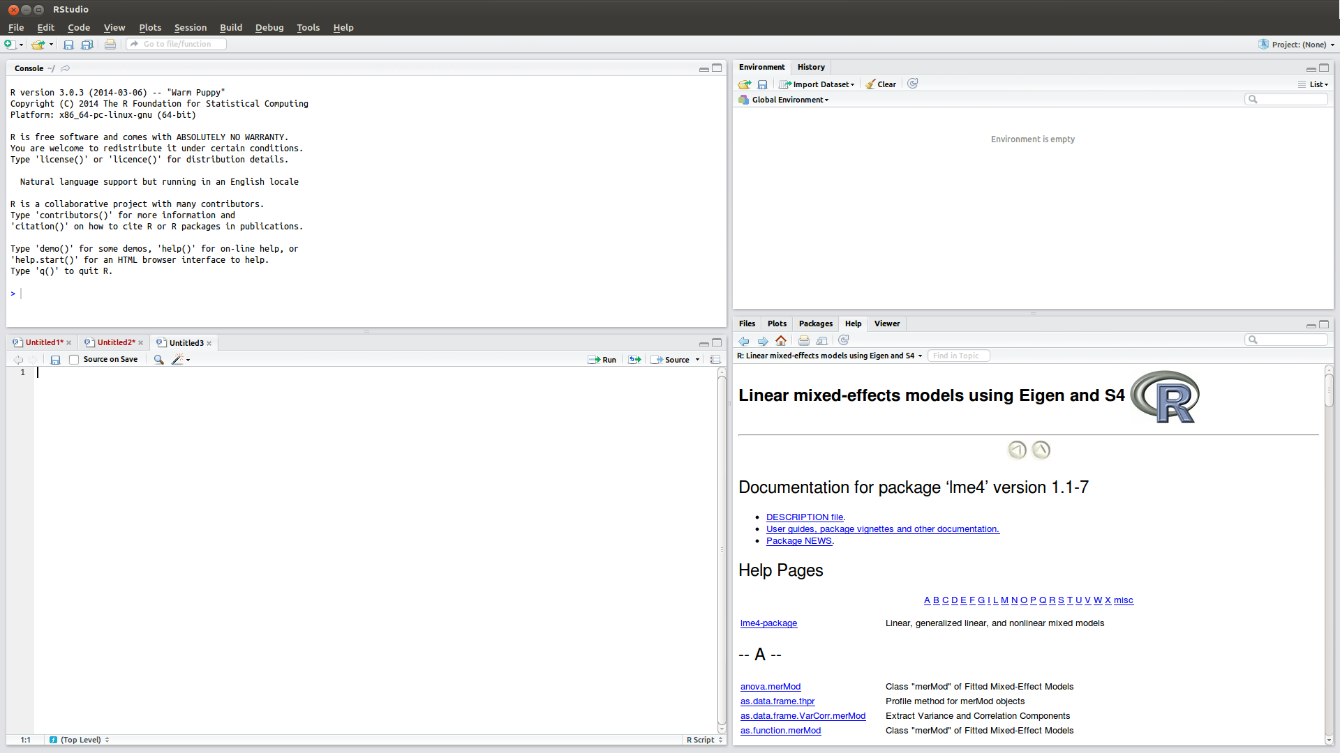
Rstudio interface (click to embiggen)

The upper left panel is an R terminal, the base around which the Rstudio program operates. The bottom left panel is an R script window, in which you can run commands into R. The upper right panel allow the user to see things like objects in the current R session (more on”objects” later). The bottom right panel includes various things like a tab for plots the user may have created and what packages are currently installed. A file browser is also there if the user wants it.

Know Where You Are in R

After understanding what you are seeing when you open an R terminal (or Rstudio), the next step is to know where R‘s working directory is. You can do this with the getwd() command. For example, my version of R in Linux has this as my default working directory.

> getwd()
[1] "/home/steve"

Windows users will see something like this.

> getwd()
[1] "C:/Users/Steve/Documents"

Windows users should notice that R, like everything else in the world, sees forward slashes (/) and not backslashes (). Windows continued use of backslashes in its file system owes to its past in DOS. Linux and Mac are derivative of Unix. Nonetheless, Windows users should note that specifying a working directory in R requires forward slashes and not backslashes.

Specifying a new working directory can be done with the the setwd() command. For example, here is my working directory for the analyses I am doing for one of my current manuscripts.

> setwd("/home/steve/Dropbox/projects/tolerance-corruption/analysis")
> getwd()
[1] "/home/steve/Dropbox/projects/tolerance-corruption/analysis"

Doing everything in Dropbox is part of a workflow talk I intend to give soon. You can specify your working directory to be whatever you want, as long as it refers to an actual directory in your file system. For example, this would give me an error.

> setwd("/home/steve/Dropbox/daves-not-here-man")
Error in setwd("/home/steve/Dropbox/daves-not-here-man") : 
  cannot change working directory

R is also case-sensitive and requires working directories to be set in quotation marks. Observe the following output.

> setwd(/home/steve)
Error: unexpected '/' in "setwd(/"
> setwd("/home/STEVE")
Error in setwd("/home/STEVE") : cannot change working directory
> setwd("/home/steve")
> getwd()
[1] "/home/steve"

Specifying a new working directory for the sake of my quantitative methods class is optional. Knowing the current working directory is important since that is where R will look for files by default and where R will save any files.

Starting to do Stuff in R

An important part to understanding R is that R is an object-oriented programming language. A helpful way of thinking about this is that input is assigned to an output using various classes and methods. For example, if I were to type hello into an R terminal for a session that I just started, I would receive this output.

> hello
Error: object 'hello' not found

This is because hello is not a built-in object in R, like, say, pi.

> pi
[1] 3.141593

I could, however, assign an input to a new object called hello. For example, I could create a vector of ten numbers drawn randomly from a normal distribution with a mean of 0 and a standard deviation of 1 as an object titled hello.

> hello  <- rnorm(10, 0, 1)
> hello
 [1]  0.002107005 -0.024397830 -0.006861523  0.538063485 -0.912956921 -1.022940134  0.075493593  0.598293193  0.190683486 -1.007443455

Or, because this is my guide on my website and I can put what I want on it:

> hello <- "annyong" 
> hello
[1] "annyong"

Be careful with what you call your objects, though.

> pi <- rnorm(10, 0, 1)
> pi
 [1]  0.10700040  0.70122694 -0.96684009 -0.48112220 -0.57755359  1.02820036 -0.51794291  0.02571443 -0.17328885 -0.10942836

Generally, you can call your objects whatever you want. Avoid naming objects things like “pi”, “T”, “TRUE”, “F”, or “FALSE”. This is an incomplete list, but hopefully it gives a student a place to start.

As a rule of thumb, I prefer shorthand in R where objects that begin with capital letters refer to data frames and objects with lower-case letters refer to variables or free-standing vectors. This is completely optional, but it helps me keep track of what are my objects in an R session.

You may also notice in my R scripts the appearance of dollar signs. In R, a dollar sign indicates a vector (i.e. a column) of a data frame. For example, looks at this line in my R script on American attitudes toward abortion in World Values Survey data.

> Data$z.age <- with(Data, (age - mean(age, na.rm = TRUE))/(2*sd(age, na.rm = TRUE)))

This means I created a new column (z.age) in a data frame (Data) that is a standardized scale of the age variable in the same data frame.

R requires assigning an input to an object with either an equal sign (=) or a left arrow (<-) to keep the object stored in the current R session. The student can always choose to not assign an output to an input if the student just wants to see something once. For example, R makes a great calculator and I find myself firing up an R session just to solve a quick math problem. Here is an example:

> 58 + 1.96*(17.8)
[1] 92.888
> 58 - 1.96*(17.8)
[1] 23.112

Installing and Loading Packages

R has hundreds upon hundreds of packages that can be installed for your use. My class will use the following packages. The install.packages() command will install these packages and whatever additional dependencies are required. In Rstudio, you can do this in the “Packages” tab located in the bottom right panel. Or, you can enter it manually into an R terminal like this.

install.packages("RCurl")
install.packages("WDI")
install.packages("countrycode")
install.packages("reshape")
install.packages("lattice")
install.packages("Zelig")
install.packages("lme4")

RCurl will allow students to read data from my Github account. WDI and countrycode are two quite useful packages created by Vincent Arel-Bundock at the University of Michigan. Respectively, they grab data from the World Bank’s data repository and convert a variety of country names into Correlates of War codes. I use these for the first problem set I assign. reshape does a variety of things, including allowing for easy renaming of columns in a data frame. lattice creates a nicer histogram than what is default in R.

Zelig and lme4 are packages that I use for the third problem set. Zelig does a variety of useful things, especially simulating of quantities of interest after estimating a statistical model. lme4 allows for the estimation of advanced mixed effects models.

It is worth reiterating that installing a package as a library and loading the package as a library for the current R session are two different things. After a package is installed, it must be loaded into the current R session. This is done with the library() command. For example, the first problem set requires the WDI, countrycode, lattice and reshape libraries.

library(WDI)
library(countrycode)
library(reshape)
library(lattice)

If you try to load a library without previously installing it, you’ll get an error message like this.

> library(RCurl)
Error in library(RCurl) : there is no package called ‘RCurl’

Running an R Script

Students in my class can visit my Github page and find one of the three repositories associated with a particular problem set I assign for homework. Each repository includes an R script that, for all intents and purposes, does the homework for the student. The student simply runs the script, sees the output, and answers the questions based off what s/he sees.

To that end, the student can save an R script from my Github by selecting on the appropriate repository, selecting the R script (with .R extension), right-clicking “Raw” and saving to the hard drive. The student can also see the input in Github and copy-paste it to an R script window in Rstudio.

From there, executing the R script from the R script window in Rstudio is straightforward. Cmd-Enter runs a line of script in Rstudio using Mac. For Linux and Windows users, this is a simple Ctrl-Enter. You can select several lines in your R script window and run them with this command as well. You can also execute the entire script with Cmd-Shift-Enter in Mac and Ctrl-Shift-Enter in Linux and Windows. For example, I ran the first few lines of the R script associated with the first problem set. This is what the output looks like. Notice the histogram in the bottom right corner.

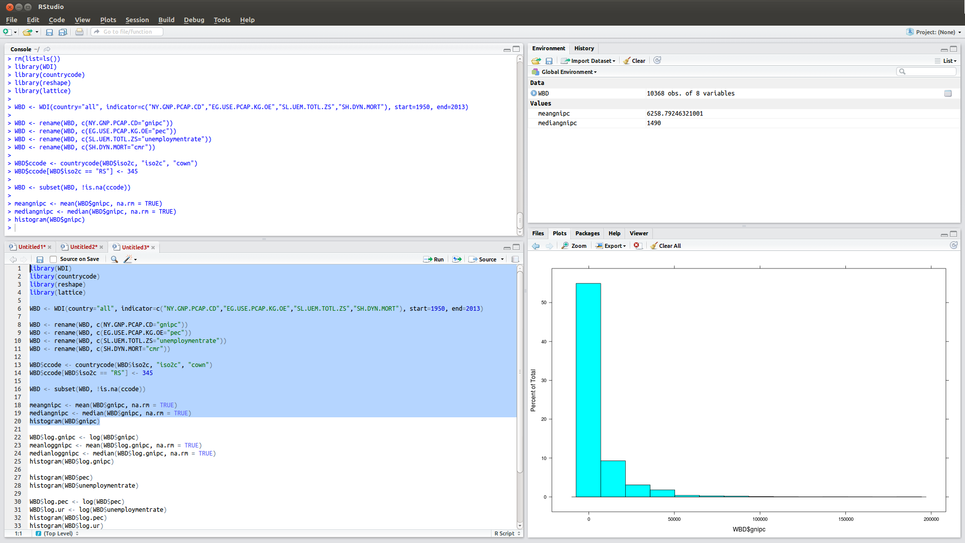
Rstudio interface (click to embiggen)

That’s really all there is to it for the sake of the classes that I teach that introduce the R programming languages. R is more daunting than it is in actuality because it is a command-line based interface. The student is encouraged to meet with me during office hours if there are still remaining questions.

Specifying a Regression Model in R

To illustrate how to do an applied statistical analysis in R, this guide will conclude with specifying a basic logistic regression. The data for this exercise will come from the Zelig package, which has a built-in data set called voteincome. Let’s call it into R.

> library(Zelig)
> data(voteincome)
> summary(voteincome)

I suppress the summary output for presentation. The reference manual for the package on CRAN provides a summary of the data. The data come from the 2000 Current Population Survey and are limited to two states (Arkansas and South Carolina) for illustration of the package. vote is a dummy variable that assumes a 1 if the respondent says she or he voted in the November 7th election.² income is an ordinal variable that ranges from 4 (makes less than $5,000) to 17 (makes more than $75,000). education is an ordinal variable that ranges from 1 (did not complete high school) to 4 (more than a college education). age and female should be self-explanatory.

Let’s look at just South Carolina for this exercise since that is where I live now. We’ll subset voteincome to just South Carolina and call it a new object Data. Recall, my preferred shorthand for objects in R is objects that begin with capital letters refer to data frames and objects with all-lower case letters refer to variables or free-floating vectors.

> Data <- subset(voteincome, state != "AR")
> summary(Data)

Let’s specify a regression model explaining an individual South Carolinian’s decision to vote in the 2000 general election. We will use all relevant predictor variables.

> M1 <- glm(vote ~ age + female + income + education, data=Data, family=binomial(link="logit"))
> summary(M1)
Call:
glm(formula = vote ~ age + female + income + education, family = binomial(link = "logit"), 
    data = Data)

Deviance Residuals: 
    Min       1Q   Median       3Q      Max  
-2.4178   0.3763   0.4540   0.5430   0.9196  

Coefficients:
             Estimate Std. Error z value Pr(>|z|)    
(Intercept) -0.331963   0.498973  -0.665 0.505864    
age          0.006639   0.005690   1.167 0.243328    
female       0.373736   0.196091   1.906 0.056659 .  
income       0.099773   0.028194   3.539 0.000402 ***
education    0.204404   0.115985   1.762 0.078013 .  
---
Signif. codes:  0 ‘***’ 0.001 ‘**’ 0.01 ‘*’ 0.05 ‘.’ 0.1 ‘ ’ 1

What we did was simple. We used the glm() function to regress vote on (i.e. ~) a linear combination of age, female, income, and education. Afterward (i.e. ,) we specified that the data to be used for the regression should come from the object we created and called Data from just the South Carolinian respondents. Then (i.e. , again) we specified the family of generalized linear model to use. We wanted logistic regression (family=binomial(link="logit")) in lieu of some other link function in the same family.

Briefly, the results suggest that gender, income, and education all have a statistically significant effect on a South Carolinian’s decision to vote in the 2000 general election. Women are more likely to vote and the more educated are more likely to vote.³ Wealthier South Carolinians are more likely to say they vote than poorer South Carolinians.

age has no statistically significant effect on voting, which is curious. What if a simple measure for age is masking a curvilinear effect? I respecified the model to include a square term for age with the I() function, which can force through a variable “as is”. This is a useful way of adding quadratic terms to a regression formula without having to create new variables that are clearly not independent of the constituent term (here: age, the most common variable in survey research that appears as a square term). My suggestion of a curvilinear effect is supported in the results that follow.

> M2 <- glm(vote ~ age + I(age^2) + female + income + education, data=Data, family=binomial(link="logit"))
> summary(M2)

Call:
glm(formula = vote ~ age + I(age^2) + female + income + education, 
    family = binomial(link = "logit"), data = Data)

Deviance Residuals: 
    Min       1Q   Median       3Q      Max  
-2.5326   0.3413   0.4231   0.5471   1.0125  

Coefficients:
              Estimate Std. Error z value Pr(>|z|)    
(Intercept) -2.7010553  0.7218704  -3.742 0.000183 ***
age          0.1320099  0.0288877   4.570 4.88e-06 ***
I(age^2)    -0.0012592  0.0002849  -4.420 9.87e-06 ***
female       0.3306201  0.1978679   1.671 0.094739 .  
income       0.0786490  0.0289024   2.721 0.006505 ** 
education    0.1940867  0.1167682   1.662 0.096482 .  
---
Signif. codes:  0 ‘***’ 0.001 ‘**’ 0.01 ‘*’ 0.05 ‘.’ 0.1 ‘ ’ 1

Here is what this curvilinear effect looks like when graphed.

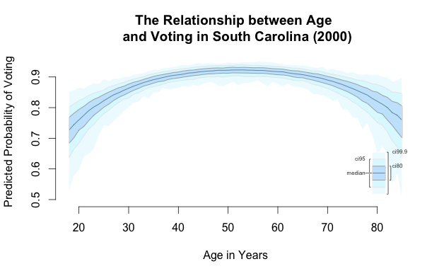
The relationship between age and voting in South Carolina (2000)