Automating a Workflow with {steveproj}, {stevetemplates}, and {targets}
- I'm easily impressed by my own parlor tricks.
I’ve been racking my brain for some time around the problem of tailoring a project’s workflow in a way that optimizes automation, reproducibility, and—depending on the project’s scale—speed. A previous stab at this looked to R Markdown as an operating system for a project. This will help link the manuscript side of a project with the analysis side of a project, but has the drawback of asking too much from R Markdown and the researcher. R Markdown really isn’t an operating system and the researcher would have to invest some time in learning about the caching and chunk quirks of R Markdown. I think I improved on this greatly with my development of {steveproj}. {steveproj} (and {stevetemplates}) have a lot of parlor tricks for preparing manuscripts, anonymized manuscripts, and title pages for peer review. However, that approach I developed last year has drawbacks in leaning hard on old school Make. It’s also a bit inflexible. It implicitly builds in a workflow that separates the analysis from the communication of the analysis, leaving not a lot of room to work interactively with the written report (as the project is still developing). Such a separation of the analysis from the report of the analysis is ideal, but never quite real.
After finally getting (somewhat) settled in Sweden, I dedicated some time to learning more about {targets}, a function-oriented Make-like tool for doing statistics in R. I think I finally figured out how to do this well in a way that’s automated, reproducible, quick, and flexible. The mechanics here are fairly simple—and my familiarity with {targets} is basic—but the approach I outline below should scale nicely. If you’re interested, I set up a basic Github repo that you can fork and run on your end to see how this works. I’ll describe it in some detail, though.
First, a table of contents.
- The Academic Project, as Concept
- The Academic Project, in Practice
- An Example Academic Project with
{steveproj},{stevetemplates}, and{targets} - Conclusion
The Academic Project, as Concept
First, I want to clarify what I believe is the basic form of most academic projects I see in my field (political science, international relations). Generally, the analysis side of a basic article-length academic project breaks into three parts. First, the project goes through a “prep” phase. The researcher loads raw data and cleans/transforms the data into a larger data object (Data) for an analysis. Thereafter, the project proceeds to an “analysis” phase. Here, the researcher estimates any number of statistical models (Mods) for the cause of assessing some cause-effect relationship. Typically, this is some sort of regression, or maybe a difference in means, but is still firmly in the inference-by-stargazing school of doing an analysis and will result in some kind of table in the project’s manuscript. Thereafter, researchers need to provide some quantities of interest (QI) from one or more of the models previously estimated. In other words, the (regression) models result in a table assessing significance of some type of causal variable while the quantities of interest communicate what the effect “looks like” to a lay audience. These could be first differences, marginal effects, model predictions, min-max effects across the range of a variable, or really anything. I almost always do this by reference to simulation from the multivariate normal distribution, given a model’s regression coefficients and variance-covariance matrix. It’s also why I think of this as the simulation (Sims) phase of the project.
No matter, there is a somewhat linear process outlined here. There are three main objects in an academic project: a data object (Data), a model object (Mods), and a (simulated) quantities of interest object (QI). The data object depends on various sources of raw data, along with assorted libraries and functions to transform/recode (“prep”) the raw data into a finished data project. The model object depends on the data object and whatever functions/libraries go into the modeling (“analysis”) phase. The quantities of interest object depends on the model object, and whatever functions/libraries go into this phase of generating (simulated) quantities of interest (“sims”).
Objects have prior (object) dependencies and functions that generate them (along with implicit dependencies on the dependencies preceding those). This type of setup can be summarized like this.
| Object | Simple (R) Function for Generating Object | Description of Object | Dependencies |
|---|---|---|---|
| Data | prep() | Generate finished data object(s) for analysis | raw data (potentially shareable), assorted libraries needed for the `prep()` function |
| Mods | analysis() | Generated (regression) model objects from an analysis | `Data`, assorted libraries needed for `analysis()` |
| QI | qi() | Generate (simulated) quantities of interest from an analysis. | `Mods`, assorted libraries needed for `qi()` |
The exact language may vary a little bit from project to project. People dealing with experimental data may be using more t-tests than sophisticated regression models. Perhaps I’m stuck in the early 2000s having fun simulating from a multivariate normal distribution of a regression model’s coefficients and variance-covariance matrix. No matter, I think this reasonably captures almost all quantitative academic projects I encounter (and certainly that I do).
And, ideally, this all happens before the researcher writes the paper describing the project. Ideally.
The Academic Project, in Practice
Ideal is never real, and the actual academic project is far more interactive and iterative than that. Perhaps the researcher first prepares the data, then analyzes the data, and gets quantities of interest from the analysis before writing the paper. Perhaps not. Perhaps the researcher is stress-testing the analysis along the way and updating the paper as they go. Perhaps they did everything in the ideal way, but the peer-review process resulted in a bunch of requests for ad hoc analyses (sorry, “robustness tests”). Perhaps the bulk of it was already written, and the results mostly communicated, but Reviewer #3 asked for another covariate in the regression model that changed nothing of substance (but requires an update to the paper regardless). In my experience, this is where the neatest and tightest of workflows starts to unravel.
It never helps that journal submission procedures are, shall we say, whimsical. Some journals are totally cool with anonymous PDFs that at least scrub the researcher’s name from the paper for the sake of double-blind peer review. Some demand peculiar formatting requirements, like separate title pages, or the absence of an abstract in the document, or whatever else. Some, monsters as they are, demand a Word document. This particular problem is primarily what motivated my development of {steveproj}.
My previous approach to this had been to lean on Make and Rscript to handle all this tedium, but that came at the expensive of interactivity for the researcher. The answer—{targets}—was always there in front of me, but it took me a while to figure out how to make it work the way I wanted to make it work. However, I think I got it now in a way that integrates {targets} into my workflow to do everything I want.
An Example Academic Project with {steveproj}, {stevetemplates}, and {targets}
My Github has an example academic project that you can clone. The contents look something like this and are inspired by the {steveproj} example I offered last year. I’ll explain the contents below.
R/: this is a repository that contains all R scripts needed for the analysis. Minimally, I think it reduces to four parts.1-prep.Rprepares data for analysis.2-analysis.Rdoes an analysis.3-qi.Rprovides so-called “quantities of interest” from the analysis. There is an additional function,_render.R, that contains all the functions for rendering documents that were otherwise in a separatesrc/directory in the previous setup. You’ll obviously want to change the contents of the first three R scripts to make them your own. In most applications, you can leave_render.Ralone.data/: this is a directory for finished data outputs. So-called “raw” data inputs that you feel are small enough to share in the project should go into a separatedata-raw/directory, if it’s appropriate. Whereas I largely deal with bigger data sets that I acquired second-hand (e.g. World Values Survey), I’m not really at liberty to include those in replication material.doc/: this is a directory for rendered documents, generated by the functions in_render.Rin theR/directory.inst/: this is an ad hoc directory that is CRAN compliant, if that interests you. You can put anything you want in there. For the sake of this simple example, I put a.bibfile for the sample manuscript that includes some citations.README.md: this is a README file._config.yaml: this is a configuration YAML file that contains what would otherwise be the YAML preamble to an R Markdown document. The value in separating this out to a separate file comes in being able to use some functions inR/_render.Rto access the same underlying information for doing things like creating an appendix or even informing the response memo to reviewers. Plus, my R Markdown parlor tricks tend to clutter the R Markdown document. Future updates of{steveproj}will make it easier to integrate a separate appendix into the project workflow, though this simple example does not include that._output.yaml: this is a simple script that tells me not to press the Knit button in Rstudio. We’ll be usingtar_make()in the{targets}package for this soon._targets.R: this is the R equivalent of a Makefile. Herein, the researcher specifies objects and dependencies. If the dependency is “newer” than the object, a command or set of commands is executed. I’ll talk more about this in the next section.ms.Rmd: this is the main manuscript describing the project. Write it as you see fit, but do notice some of the parlor tricks in there that do things like conditional rendering of tables and figures contingent on whether the output is a LaTeX PDF or a Word document.
_targets.R: The R Corollary to a Makefile
This is the contents of a simple _targets.R file to serve as the basic operating system for an academic project. At various points below, I’ll annotate what the code is doing.
# load {targets} library
library(targets)
# source all files in the R/ directory
sapply(list.files("R", full.names=TRUE), source)
# ^ you could alternatively do this manually, like so:
# source("R/1-prep.R")
# source("R/2-analysis.R")
# source("R/3-qi.R")
# source("R/_render.R")
# Below: as global option, load packages you'll need for executing the scripts
tar_option_set(packages = c("stevedata", "tidyverse", "modelr", "stevemisc"))
# Now, time to specify our targets and dependencies...
list(
  # for example, the object Data depends on the prep() function that creates it.
  # if prep() is "newer" than Data, prep() is executed.
  tar_target(Data, prep()),
  # Likewise, Mods has two dependencies: Data and analysis().
  tar_target(Mods, {
    Data
    analysis()
    }),
  # The quantities of interest depend on the data and model object, and also qi()
  tar_target(QI, {
    Mods
    Data
    qi()
  }),
  # specialty targets: the .Rmd and YAML are flat files
  tar_target(ms_rmd, "ms.Rmd", format = "file"),
  tar_target(ms_yaml, "_config.yaml", format = "file"),
  # Finally, docs is a target for the document outputs.
  # If anything in the brackets is changed, the document outputs are changed too.
  tar_target(docs, {Data
    Mods
    QI
    ms_rmd
    ms_yaml
    render_pdf() # <- render nice-looking PDF
    render_pdfanon() # <- render anonymous PDF
    render_docx() # <- render (anonymous) Word document
    })
)
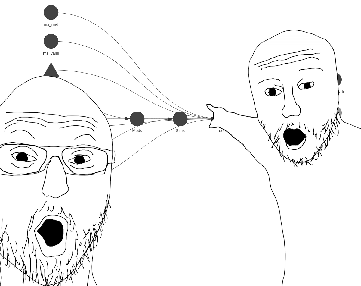
If you remember the previous {steveproj} post, the mechanics of what’s happening here should seem familiar. Again, it’s an R corollary to Make, with the benefit of being native to R. This means you can do the same thing as a Makefile without leaving the current environment to have a Makefile execute standalone R scripts (as I was previously doing). Plus, it comes with a handy tool for visualizing the project’s workflow.
library(targets) # load {targets} into session for good measure
tar_visnetwork()
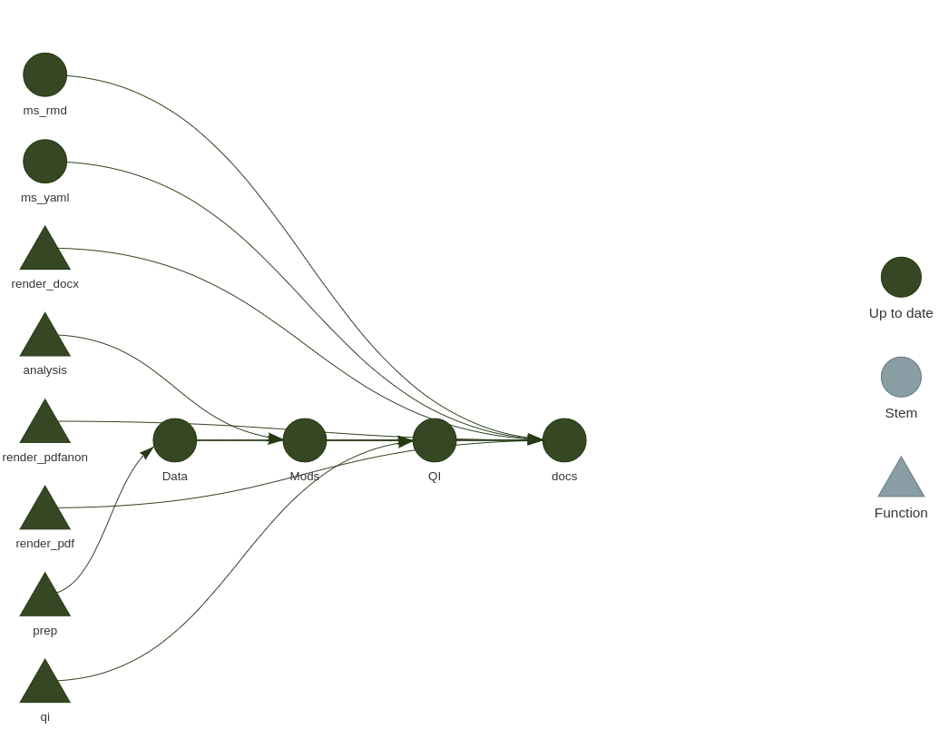
- A pipeline dependency graph of the academic project
This function isn’t necessary for the project to execute, but it’s a nifty diagnostic tool as the project grows in complexity. It’ll also identify errors you may have made specifying dependencies.
R Scripts as “Functions” and Not “Scripts”, and the Power of “Superassignment”
One of the biggest oddities for me wrapping my head around {targets} was the idea that the project should consist of “functions”, and not multiple scripts for generating various outputs. Notice the above _targets.R file references functions of prep(), analysis(), and qi(). These are not native to R, {tidyverse}, any of my functions in my packages, or really anything else in a prominent R package. These are R functions you have to write yourself to do whatever it is you want to do.
Again, this seemed very strange to me, especially thinking of custom R functions that should be CRAN-compliant. However, these functions don’t need to be CRAN-compliant. They can be whatever you want them to be with that in mind. And, with that in mind, perhaps what I saw as a “script” was itself a function by another name.
Consider the contents of 1-prep.R as a simple example of what’s happening here, and what might be an advisable track for your workflows with {targets}.
prep <- function() {
  set.seed(8675309)
  ESS9GB %>%
    mutate(noise = rnorm(nrow(.))) -> Data

  saveRDS(Data, "data/Data.rds")
  Data <<- Data
  return(Data)
}
If you were to strip away the prep <- function() {} wrapper, this would look like a simple R script, even if it implicitly assumed you had loaded {tidyverse} and {stevedata} for the underlying data and some other functions (e.g. mutate() and the pipe operator). However, the simple R script is getting wrapped in a function, named prep(), that has no arguments. When called, it simply executes the contents of the function. The application here is very simple and depend on libraries declared near the top of the _targets.R file. It starts with my favorite reproducible seed. It takes a “raw” data set, ESS9GB, that is in {stevedata} and you can read more about on my blog. It prepares a “finished” data output, titled Data, that is a simple random noise variable amended to the raw data. It then saves Data to the data/ folder in the project’s directory.
I do want to call attention to a little used assignment operator that is incredibly useful for a purpose like this. The double arrow (<<-) “superassignment” operator, when called into a function, has the effect of placing the object into the global environment. This is a neat trick for working interactively with a project in R, because the normal assignment operator would not do this. Observe this simple case, an effective reproduction of what’s happening above. In the first case, the function is doing what it should. It creates an object, Data, and displays it into the session though the referenced object, Data, is not placed in the global environment. In the second case, double-arrow “superassignment” returns the created Data object into the session and as an object in the global environment.
mtcars_data <- function() {
  Data <- head(mtcars, 5)
  return(Data)
}

mtcars_data()
#>                    mpg cyl disp  hp drat    wt  qsec vs am gear carb
#> Mazda RX4         21.0   6  160 110 3.90 2.620 16.46  0  1    4    4
#> Mazda RX4 Wag     21.0   6  160 110 3.90 2.875 17.02  0  1    4    4
#> Datsun 710        22.8   4  108  93 3.85 2.320 18.61  1  1    4    1
#> Hornet 4 Drive    21.4   6  258 110 3.08 3.215 19.44  1  0    3    1
#> Hornet Sportabout 18.7   8  360 175 3.15 3.440 17.02  0  0    3    2
Data
#> Error in eval(expr, envir, enclos): object 'Data' not found

# Now, with superassignment.
mtcars_data <- function() {
  Data <<- head(mtcars, 5)
  return(Data)
}

mtcars_data()
#>                    mpg cyl disp  hp drat    wt  qsec vs am gear carb
#> Mazda RX4         21.0   6  160 110 3.90 2.620 16.46  0  1    4    4
#> Mazda RX4 Wag     21.0   6  160 110 3.90 2.875 17.02  0  1    4    4
#> Datsun 710        22.8   4  108  93 3.85 2.320 18.61  1  1    4    1
#> Hornet 4 Drive    21.4   6  258 110 3.08 3.215 19.44  1  0    3    1
#> Hornet Sportabout 18.7   8  360 175 3.15 3.440 17.02  0  0    3    2
Data
#>                    mpg cyl disp  hp drat    wt  qsec vs am gear carb
#> Mazda RX4         21.0   6  160 110 3.90 2.620 16.46  0  1    4    4
#> Mazda RX4 Wag     21.0   6  160 110 3.90 2.875 17.02  0  1    4    4
#> Datsun 710        22.8   4  108  93 3.85 2.320 18.61  1  1    4    1
#> Hornet 4 Drive    21.4   6  258 110 3.08 3.215 19.44  1  0    3    1
#> Hornet Sportabout 18.7   8  360 175 3.15 3.440 17.02  0  0    3    2
This may not seem like much, but it’s going to be very useful for executing the functions interactively, and into the R session, without having to manually do something like Data <- readRDS("data/Data.rds"). Should you pivot your workflow to {targets}, you may want to consider using the double-arrow “superassignment” operator in all your functions.
Putting Everything Together (i.e. Drawing the Rest of the Owl)
The example I provide is a simple toy example. Perhaps at another time, or maybe as a book project, I can unpack what’s happening in the _render.R function where I manually create some temp files from glueing the YAML and Rmd files together. However, you can draw the rest of the owl by doing one of a number of things.
First, if you wanted to execute the project as if it were a Makefile, you’d run tar_make() in the R session.
library(targets)
tar_make()
The above tar_make() call executes the prep(), analysis(), and qi() functions to create their appropriate targets. It also executes the various “render” functions in R/_render.R to create the documents in doc/, though I’m assuming you know at least a little about R Markdown by this point.
However, tar_make() kind of assumes the project is “done”, at least as I’ve written it. If you were still tweaking the project, like estimating different models or still cleaning the data, you could still use {targets} for an interactive session. For one, tar_load_globals() loads globals for debugging and testing. This has the effect of loading the global options and loading the custom functions sourced in _targets.R.
tar_load_globals()
Thereafter, you can call the custom functions you’ve written—here: prep(), analysis(), and qi(). You can see this for yourself in the Environment tab in Rstudio.
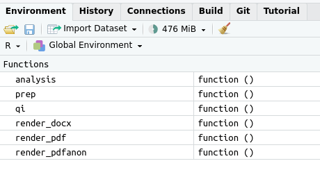
- tar_load_globals() loads the libraries and the functions into the current R session.
Thereafter, you can call them individually in the R session, as you see fit.
prep()
analysis()
qi()
If you’re still writing the manuscript and like to do periodic updates to check your work, you can render the PDF to see how it looks.
render_pdf()
Conclusion
The Github repository with this simple example is enough to get started. It’s a far cry from what any researcher will end up doing, but that’s also not the point of a simple example designed to illustrate what is possible. Going forward, {steveproj} will do this as a kind of default. It will also include simple functions to extend the workflow with separate documents like an appendix or a response memo. All that said, if you can root your R project in {targets}, you should. {stevetemplates} will allow for some parlor tricks with R Markdown and {steveproj} will be a wrapper for all this, but {targets} is the workhorse here. You should invest time in learning its basics because the payoff is worth it.
Disqus is great for comments/feedback but I had no idea it came with these gaudy ads.