An Illustration of Decision Trees and Random Forests with an Application to the 2016 Trump Vote
- A not so random forest
I’m writing this mostly as a guide to teach myself some more statistical modeling parlor tricks. In this application, I’ve never taken the time to sit down and learn the class of techniques at the core of what we call “machine learning.” These techniques may ultimately be a fancier way of saying “regression” in a lot of applications, but they have some properties that are useful for their intended task and audience: prediction.1 This is a goal for those working in the private sector more interested in predicting outcomes and less interested in “explaining” them, per se (even if that comes off as a false dichotomy). No matter, they’re not techniques you’ll pick up in the social sciences, which is more interested in “explanation” and causal identification than prediction.2 They’re also techniques that I should demonstrate I know given the current pandemic and threats to higher education in the United States.
Toward that end, I’m going to walk myself through some rudimentary things in the machine learning context: decision trees and random forests. I’m going to use a data set intimately familiar to me: the individual-level Trump vote in 2016. I’ve used these data elsewhere on my blog looking at ordinal modeling of attitudes toward cognitive racism, and straight-up modeling of the Trump vote in 2016 in the Midwest and nationwide. In this application, I’m going to set up a decision tree model and a random forest model of the Trump vote among white voters, starting with a focus on some Midwestern states. Here are the R packages I’ll be using in this analysis.
library(stevemisc) # my toy R package
library(stevedata) # for the data
library(tidyverse) # for most things
library(modelr) # for some partitioning stuff.
library(knitr) # for tables
library(kableExtra) # for pretty tables
library(randomForest) # for randomForest
And here’s a table of contents.
The Data
I’m not going to belabor the data here as I’ve belabored them elsewhere, but I’m going to do a handful of things here. First, for convenience sake, I’m going to create some variable labels for the data I’ll be using. I do this quietly (check the relevant .Rmd in the _rmd directory), but here’s a summary of the model inputs to explain the Trump vote.
| Variable | Variable Label |
|---|---|
| age | Age in Years |
| female | Respondent Identifies as Female (Y/N) |
| collegeed | Respondent Has Four-Year College Diploma (Y/N) |
| famincr | Household Income [1:12] |
| ideo | Ideology [Very Liberal:Very Conservative, 1:5] |
| pid7na | Partisanship [Strong D:Strong R, 1:7] |
| bornagain | Respondent is Born-Again Christian (Y/N) |
| religimp | Importance of Religion to Respondent [1:4] |
| churchatd | Rate of Church Attendance for Respondent [1:6] |
| prayerfreq | Reported Frequency of Prayer for Respondent [1:7] |
| angryracism | Respondent is Angry Racism Exists [Strongly Agree:Strongly Disagree, 1:5] |
| whiteadv | White People Have Advantages Over Others [Strongly Agree:Strongly Disagree, 1:5] |
| fearraces | Respondent Fears Other Races [Strongly Disagree:Strongly Agree, 1:5] |
| racerare | Respondent Thinks Racism is Rare [Strongly Disagree:Strongly Agree, 1:5] |
Now, let’s set up a data set of just white voters in the Midwest in these 2016 survey data. I’m also going to start this data-cleaning process with the usa_states data frame in my {stevedata} package. This is a simple data set that also includes Census region identifiers, which will be useful for some machine learning stuff down the road in this analysis.
# Your classification of the Midwest may vary. This is the forever war of Midwest Twitter/Reddit.
midwest_states <- c("Iowa", "Minnesota", "Wisconsin", "Ohio", "Pennsylvania", "Michigan",
                   "Wisconsin", "Illinois", "Indiana")

# ^ If you're curious, this is basically classic Big Ten + Pennsylvania for good measure.

usa_states %>%
  # select State name and Census region
  select(statename, region) %>%
  rename(state = statename) %>%
  left_join(TV16, .) -> TV16

TV16 %>%
  # select just those respondents in midwest_states
  filter(state %in% midwest_states) %>%
  # then: select just those who self-identify as white
  filter(racef == "White") %>%
  # Let's drop either some constants (e.g. racef), new variables I created elsewhere (e.g. lemprac), and other identifiers.
  select(-racef, -lrelig, -lcograc, -lemprac, -uid, -state, -region) %>%
  # machine learning stuff hates characters, likes factors, whereas Steve generally hates factors, likes characters
  # different audience, different aims, tho...
  mutate_if(is.character, as.factor) %>%
  # recode partisanship to factor for clarity sake
  mutate(pid7na = dplyr::recode_factor(pid7na, `1` = "Strong D",
                                       `2` = "Not Strong D",
                                       `3` = "Ind. Lean D",
                                       `4` = "Independent",
                                       `5` = "Ind. Lean R",
                                       `6` = "Not Strong R",
                                       `7` = "Strong R",
                                       .ordered = TRUE)) %>%
  # The racism variables are handled a bit differently.
  mutate_at(vars("whiteadv","angryracism"), ~dplyr::recode_factor(.,
                                  `1` = "Strongly Agree",
                                  `2` = "Agree",
                                  `3` = "NA/ND",
                                  `4` = "Disagree",
                                  `5` = "Strongly Disagree",
                                  .ordered = TRUE)) %>%
  # Put the thing down flip it and reverse it
   mutate_at(vars("fearraces","racerare"), ~dplyr::recode_factor(.,
                                  `1` = "Strongly Disagree",
                                  `2` = "Disagree",
                                  `3` = "NA/ND",
                                  `4` = "Agree",
                                  `5` = "Strongly Agree",
                                  .ordered = TRUE))-> Midwest
Next, let’s partition the data. Machine learning people have several means to validate their predictive models, but a fairly boilerplate approach here is to split the data into a “training” set and a “testing” set. Therein, the model predicts/”learns” on the training set and insights from the training model can then be applied to the testing set to assess model performance. I’ve yet to see any hard rules for how to approach training and testing partitions, but I routinely see data split 80%/20% training/testing. It’s not hard to do with {modelr}.
set.seed(8675309) # Jenny, I got your number...
Midwest %>%
  resample_partition(p = c(test = 0.2, train = 0.8)) -> Partition

Partition %>%
  pluck("train") %>%
  as_tibble() -> Train

Partition %>%
  pluck("test") %>%
  as_tibble() -> Test
From here, we can engage in any number of machine learning models. We’ll start with a basic decision tree.
A Decision Tree Approach
A decision tree assigns labels to individual observations, separating individual observations in the data set into subsets that are increasingly likely to share the same class label. The presentation of this flowchart is “tree-like”, hence the name. One quirk about a straightforward decision tree approach is there is no globally optimal way of doing it, and so decision tree models typically employ a “locally optimal” strategy in a recursive partitioning approach. In the absence of any split where all observations belong to a single class, the data are split in a way in which the “purity” exceeds some threshold. The most popular method on this front might be the Gini coefficient, though information gain is another common approach.
A researcher can implement a decision tree quite simply with the rpart() function in the {rpart} package.
mDT <- rpart::rpart(as.factor(votetrump) ~ ., data = Train)
The more I have played with this approach, the less I like it. I have my reasons. First, the top of the tree gives the single best split for the training data set. I worry this implies that identifying that single “best” split is a function of the composition of the training set. Even asking for more trees doesn’t change what split appears at the top. Thus, the researcher may encounter a top node of the tree that is completely unintuitive from a theoretical perspective. In a somewhat simple application like what I have here, the top node is going to be easy to understand. Perhaps, then, a simple decision tree approach is elegant for outcomes that can be predicted by relatively simple relationships.
Second, there’s just something about the presentation of these models that I find to be unhelpful. This isn’t about the components of the model, but the implementation and presentation of it in the {rpart} package. The summary() function just produces a stream of output. Calling the object (here: mDT) in the R session gives you more of what you want, but it’s also unintuitive.
mDT
#> n=7523 (2414 observations deleted due to missingness)
#>
#> node), split, n, loss, yval, (yprob)
#>       * denotes terminal node
#>
#>  1) root 7523 3535 0 (0.53010767 0.46989233)
#>    2) pid7na=Strong D,Not Strong D,Ind. Lean D 3394  308 0 (0.90925162 0.09074838) *
#>    3) pid7na=Independent,Ind. Lean R,Not Strong R,Strong R 4129  902 1 (0.21845483 0.78154517)
#>      6) pid7na=Strong D,Not Strong D,Ind. Lean D,Independent 1021  508 0 (0.50244858 0.49755142)
#>       12) whiteadv=Strongly Agree,Agree 384   91 0 (0.76302083 0.23697917) *
#>       13) whiteadv=NA/ND,Disagree,Strongly Disagree 637  220 1 (0.34536892 0.65463108) *
#>      7) pid7na=Ind. Lean R,Not Strong R,Strong R 3108  389 1 (0.12516088 0.87483912) *
You can graph it as well.
plot(partykit::as.party(mDT))
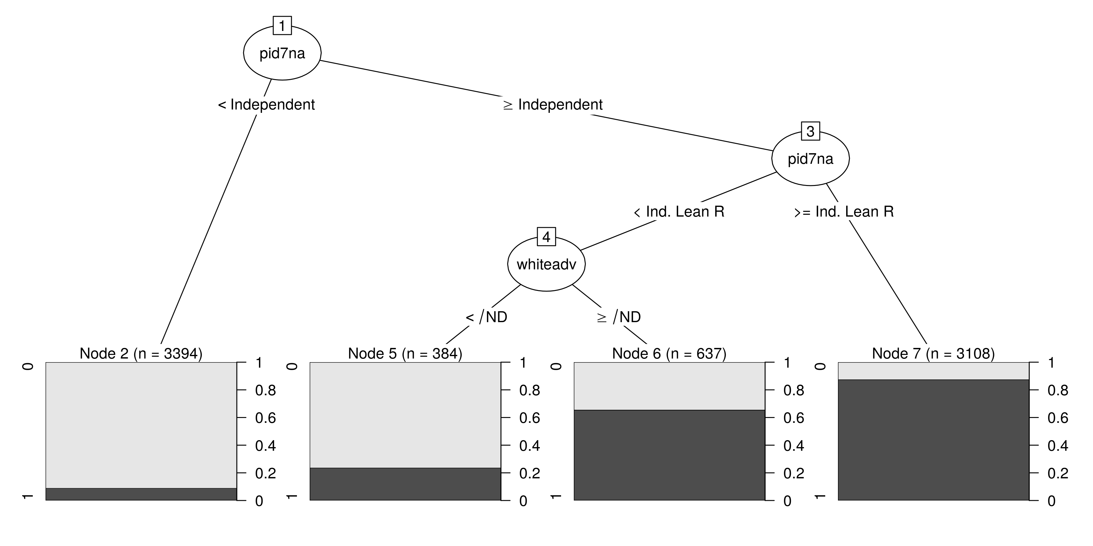
This is where some subject expertise is not only handy, but necessary in the machine learning context. The model output implies that the white vote for Donald Trump in the Midwest is most easily predicted by just two things: partisanship and the respondent’s attitudes about the structural advantages for white people relative to non-white people. Generally, echoing my previous analyses on the Trump vote in 2016 in the Midwest and nationwide, the takeaway here seems to be that you only need two things to understand the Trump vote in the Midwest: partisanship and attitudes on race. More than that, the effect of increasing racial bias among white voters on their likelihood of voting for Trump is seemingly stronger among Democrats and Democratic leaners than the effect of decreasing racial bias was among Republicans and Republican leaners.
A Random Forest Approach
Again, there’s just something about the decision tree approach that I don’t quite like from a perspective more attuned to classical “statistics.” I could always play with some of the tuning parameters to create more complex trees, and this may or may not help with the overall goal of prediction and accuracy. Still, my major misgivings with this approach in R are the deterministic nature of the first split (even as it makes perfect sense in a simple case like this) and the somewhat awkward presentation of it.
Random forests are a natural extension of the decision tree approach and they appeal quite nicely to my background in sampling. Random forests are “bagging” approaches to machine learning, in that they are a combination of bootstrapping and model aggregation. This sounds awfully convoluted if you’re first trying to learn this stuff, but, if you know bootstrapping, you’ll pick up on this pretty quickly. tl;dr: a random forest is constructed by bootstrapping (with replacement) the original data set into a given number of samples, selecting only a handful of inputs, and building a decision tree from that individual bootstrapped data set.
The randomForest() command in the {randomForest} package will do this, where ntree is the number of bootstrapped samples and mtry is the number of inputs to include in a particular bootstrapped sample. Random forests are nifty, but can be computationally expensive. So, the number of trees should be reasonable to make sure every row is sampled, but asking for a million trees is going to bottleneck the R session with potentially no real payoff.
set.seed(8675309) # Jenny, I got your number...
mRF <- randomForest(as.factor(votetrump) ~ .,
                    data=Train,
                    ntree=500, # 500 is default
                    mtry = 3, # can't be more than 14 (the number of inputs I have). Let's try 3.
                    oob_score = TRUE,
                    na.action = na.exclude)
Random forests don’t have the deterministic limitations of the decision-tree approach, nor do they have that kind of top-down visual interpretation. In our model, it should make sense that any decision tree model of the Trump vote that includes partisanship is going to start with partisanship because it’s the single most important predictor of a partisan vote in American politics, but, in this random forest model, there is no guarantee that partisanship is even included in the particular sample. So, there could be some other first split.
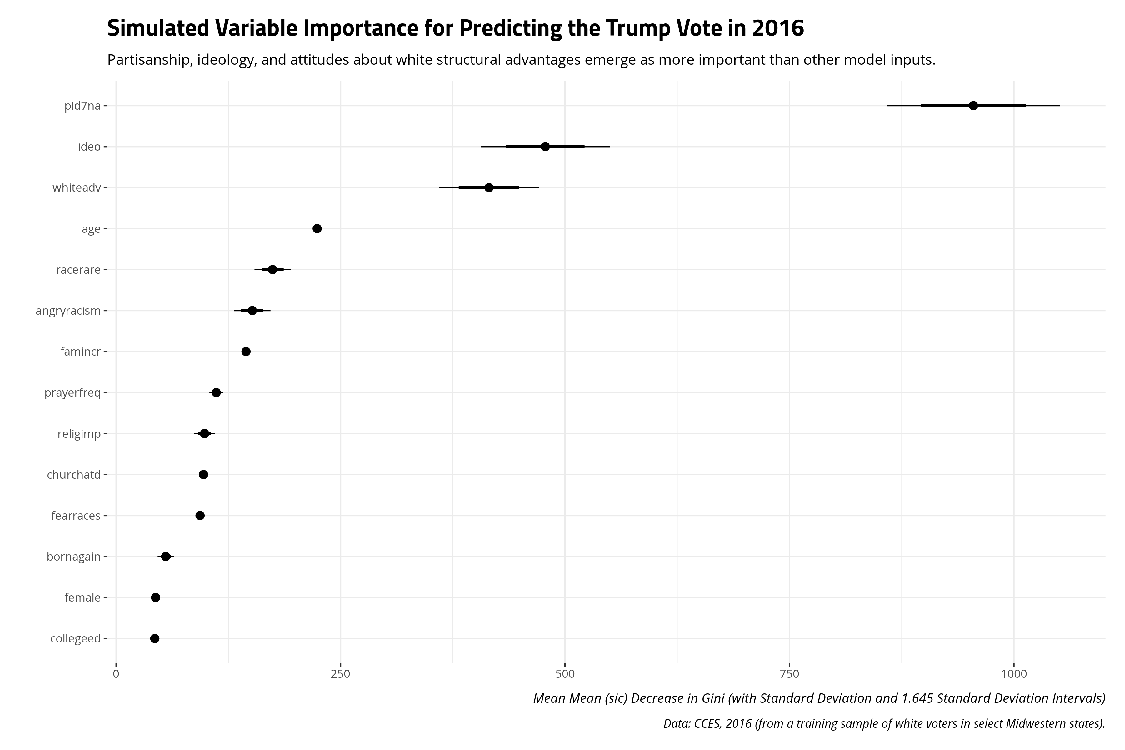
Instead of looking for a first split, it makes more sense to summarize a random forest first by the “importance” of the inputs. Recall that random forests are an ensemble of individual decision trees. Gini importance can be leveraged from these individual decision trees to calculate a mean decrease in Gini, which is the average of a variable’s total decrease in node impurity, weighted by the proportion of samples reaching that node in each individual decision tree in the random forest. It emerges as a measure of how “important” a variable is for estimating the outcome variable of interest. Higher values indicate greater variable “importance.”
importance(mRF) %>% as_tibble() %>%
  mutate(var = rownames(importance(mRF))) %>%
  # Don't like having to do it this way, but alas...
  select(2, 1)
| Variable Label | Mean Decrease in GINI |
|---|---|
| Partisanship [Strong D:Strong R, 1:7] | 963.53 |
| Ideology [Very Liberal:Very Conservative, 1:5] | 454.38 |
| White People Have Advantages Over Others [Strongly Agree:Strongly Disagree, 1:5] | 419.87 |
| Age in Years | 224.70 |
| Respondent Thinks Racism is Rare [Strongly Disagree:Strongly Agree, 1:5] | 172.91 |
| Respondent is Angry Racism Exists [Strongly Agree:Strongly Disagree, 1:5] | 155.44 |
| Household Income [1:12] | 144.68 |
| Reported Frequency of Prayer for Respondent [1:7] | 113.75 |
| Importance of Religion to Respondent [1:4] | 101.43 |
| Rate of Church Attendance for Respondent [1:6] | 97.18 |
| Respondent Fears Other Races [Strongly Disagree:Strongly Agree, 1:5] | 93.05 |
| Respondent is Born-Again Christian (Y/N) | 56.17 |
| Respondent Has Four-Year College Diploma (Y/N) | 44.16 |
| Respondent Identifies as Female (Y/N) | 43.35 |
It should be no surprise that partisanship emerges as having the largest importance for estimating the target variable. The next most important inputs are the respondent’s ideology, and then the white advantage prompt that emerged as the only other split in the decision tree approach. This is a slight departure from the decision tree model. The decision tree model suggested it really did not need to know the respondent’s ideology more than attitudes about white advantage for the sake of making predictions.
One limitation of variable importance is that there is no formal inferential component to the average decrease in Gini. This makes it useful for developing hypotheses, but not super useful for making comparisons, or at least making comparisons with some kind of precision or confidence. I wonder if one way around this is to continue the boostrapping approach, of sorts, by repeating the process and summarizing the measures of variable importance that come from it. Here is a simple illustration.
importance_tab <- as_tibble()

set.seed(8675309) # Jenny, I got your number...
for (i in 1:100) {
  mod <- randomForest(as.factor(votetrump) ~ ., data=Train,
                      # Let's do 100 just to speed this up.
                      ntree=100, mtry = 3, na.action = na.omit)
  hold_this <- importance(mod) %>% tbl_df() %>%
    mutate(var = rownames(importance(mod)), num = i)
  importance_tab <- bind_rows(importance_tab, hold_this)
}
To be clear, I offer this with some hesitation because I’ve seen no one do this before and there’s still no “null hypothesis” to consider here. But alas, you could do this.
Assessing Model Performance
There are a number of ways to assess model performance, but a modeler most interested in prediction will probably start with an assessment of the model’s predictive accuracy. In the machine learning context, this is called a “confusion matrix.” This is, to be polite, an unintuitive way of naming a procedure that looks at model predictions to determine how often they’re correctly predicting the observed 0s and 1s, but that’s what it really is. The “confusion matrix” is a 2x2 table that communicates 1) the observed 0s that were predicted to be 0 [correct], 2) the observed 0s that were predicted to be 1 [incorrect], 3) the observed 1s that were predicted to be 0 [also incorrect], and 4) the observed 1s that were predicted to be 1 [correct].
So, let’s do a series of these forms of model assessment. First, we’ll calculate confusion matrices for the training data with predictions derived from the decision tree model and the random forest model. Then, we’ll get predictions on the testing data of white, Midwestern respondents. These are observations that did not inform the decision tree model or random forest model and thus could be used for this kind of task. Thereafter, we’ll go even further out of sample to assess how well our training data of white, Midwestern voters does in explaining the vote choice of white respondents in other states that did not comprise the sample.
Let’s start with the comparison of predictive accuracy for the white respondents in these select Midwestern states, looking at the training data and testing data, by model.
# Some null predictions first...
mNull1 <- glm(as.factor(votetrump) ~ 1, data=Train, family=binomial)
mNull2 <- glm(as.factor(votetrump) ~ 1, data=Test, family=binomial)

# Training predictions: Null
Train %>%
  mutate(pred = predict(mNull1, type="response", newdata=.)) %>%
  select(votetrump, pred) %>%
  # I already know what this is going to do...
  mutate(pred = ifelse(pred < .5, 0, 1)) %>%
  mutate(category = "Training: Null Model") -> predTrainNM

# Training predictions: DT
Train %>%
  mutate(pred = predict(mDT,type="class", newdata=.)) %>%
  select(votetrump, pred) %>%
  mutate(pred = as.numeric(pred)-1) %>%
  mutate(category = "Training: Decision Tree") -> predTrainDT

# Training predictions: RF
Train %>% na.omit %>%
  mutate(pred = mRF$predicted) %>%
  # If you do it the way below, you're going to perfectly predict almost everything...
  # mutate(pred = predict(mRF, newdata=., type="class")) %>%
  select(votetrump, pred) %>%
  mutate(pred = as.numeric(pred)-1) %>%
  mutate(category = "Training: Random Forest") -> predTrainRF

Test %>%
  mutate(pred = predict(mNull2, type="response", newdata=.)) %>%
  select(votetrump, pred) %>%
  # I already know what this is going to do...
  mutate(pred = ifelse(pred < .5, 0, 1)) %>%
  mutate(category = "Testing: Null Model") -> predTestNM

# Testing predictions: DT
Test %>%
  mutate(pred = predict(mDT,type="class", newdata=.)) %>%
  select(votetrump, pred) %>%
  mutate(pred = as.numeric(pred)-1) %>%
  mutate(category = "Testing: Decision Tree") -> predTestDT

# Testing predictions: RF
Test %>%
  mutate(pred = predict(mRF, newdata=.)) %>%
  select(votetrump, pred) %>%
  mutate(pred = as.numeric(pred)-1) %>%
  mutate(category = "Testing: Random Forest") -> predTestRF

bind_rows(predTrainNM, predTrainDT, predTrainRF, predTestNM, predTestDT, predTestRF) %>%
  group_by(category, votetrump, pred) %>%
  count() %>% na.omit %>%
  group_by(category) %>%
  mutate(totaln = sum(n),
         correct = ifelse(votetrump == pred, 1, 0)) %>%
  filter(correct == 1) %>%
  summarize(accuracy = sum(n)/first(totaln)) %>%
  separate(category, c("Data", "Model"), sep=": ") %>%
  # I'd rather do it this way than make it a factor...
  slice(5,4,6,2,1,3)  -> accuracyTT
| Data | Model | Accuracy |
|---|---|---|
| Training | Null Model | 0.530 |
| Training | Decision Tree | 0.866 |
| Training | Random Forest | 0.879 |
| Testing | Null Model | 0.541 |
| Testing | Decision Tree | 0.871 |
| Testing | Random Forest | 0.895 |
The results suggest a simple decision tree model and a simple random forest model both do well to correctly predict the observed Trump vote values in this sample of white respondents in these select Midwestern states. There is a slight advantage to the random forest model, which has better predictive accuracy for both the training data and, importantly, the testing data. No matter, the difference is slight and the predictive accuracy is still over 85% no matter the model and data. Both certainly do better than the null model, which predicts no one votes for Donald Trump in these Midwestern states. That null model is accurate just about 55% of the time.
We could also assess model accuracy by doing an out of sample prediction of a sort. We trained two models on a subset of white respondents in some select Midwestern states. We tested on additional white respondents in these same Midwestern states that did not comprise the training data. We can go further and test our predictions on respondents in other states not included in the training data.
TV16 %>%
  filter(racef == "White" & state %nin% midwest_states) %>%
  # gotta do this again...
  mutate_if(is.character, as.factor) %>%
  # recode partisanship to factor for clarity sake
  mutate(pid7na = dplyr::recode_factor(pid7na, `1` = "Strong D",
                                       `2` = "Not Strong D",
                                       `3` = "Ind. Lean D",
                                       `4` = "Independent",
                                       `5` = "Ind. Lean R",
                                       `6` = "Not Strong R",
                                       `7` = "Strong R",
                                       .ordered = TRUE)) %>%
  # The racism variables are handled a bit differently.
  mutate_at(vars("whiteadv","angryracism"), ~dplyr::recode_factor(.,
                                  `1` = "Strongly Agree",
                                  `2` = "Agree",
                                  `3` = "NA/ND",
                                  `4` = "Disagree",
                                  `5` = "Strongly Disagree",
                                  .ordered = TRUE)) %>%
  # Put the thing down flip it and reverse it
   mutate_at(vars("fearraces","racerare"), ~dplyr::recode_factor(.,
                                  `1` = "Strongly Disagree",
                                  `2` = "Disagree",
                                  `3` = "NA/ND",
                                  `4` = "Agree",
                                  `5` = "Strongly Agree",
                                  .ordered = TRUE)) %>%
  group_split(state) %>%
  map(~mutate(., pred_null = predict(glm(as.factor(votetrump) ~ 1, data=., family=binomial), type="response", newdata=.),
              pred_null = ifelse(pred_null < .5, 0, 1),
              pred_rf = predict(mRF, newdata=.),
              pred_dt = predict(mDT, newdata = ., type="class"))) %>%
  map(~select(.,state, votetrump, pred_null, pred_rf, pred_dt)) %>%
  map_df(., bind_rows) %>%
  gather(model, pred, 3:5, -state, -votetrump) %>%
  mutate(pred = as.numeric(pred)) %>%
  na.omit %>%
  group_by(state, model) %>%
  mutate(totaln = n(),
         correct = ifelse(votetrump == pred, 1, 0)) %>%
  filter(correct == 1) %>%
  summarize(accuracy = sum(correct)/first(totaln)) %>%
  ungroup() %>%
  mutate(model = case_when(model == "pred_null" ~ "Null Model",
                           model == "pred_dt" ~ "Decision Tree",
                           model == "pred_rf" ~ "Random Forest")) -> accuracyStates
The following graph compares the predictive accuracy of the null model (green triangle), the decision tree (red circle), and the random forest (blue square) for predicting the Trump vote among white voters in states not included in the training data. Overall, training two models on white voters in some select Midwestern (i.e. Big Ten) states does comparably well in predicting the white Trump vote in out of state samples as it does on testing data in these same states. That is: the inputs that predict the white Trump vote in those states generally port well to other state contexts. There are three exceptions, though. First, Idaho and especially Utah stand out as having much lower predictive accuracy than every other state. The predictive accuracy of the decision tree model and the random forest model hover around the mid-to-high 80s (and even the low 90s in some states like South Carolina). However, the predictive accuracy in Idaho is in the low 80s and the predictive accuracy in Utah is low-to-mid 70s. Thinking of the Utah case, in particular, it suggests there are either 1) missing inputs, unique to these contexts, that could help explain what the model is missing relative to other contexts and/or 2) that features included in the training model might not have the same kind of effect in Utah as they have in almost every other context. Subject domain expertise of the political attitudes of white people in Idaho and Utah may help tailor a predictive model to explain those observations. Subject domain expertise will also caution that training on white Midwestern respondents to predict attitudes in Idaho and Utah is going to miss some important things.
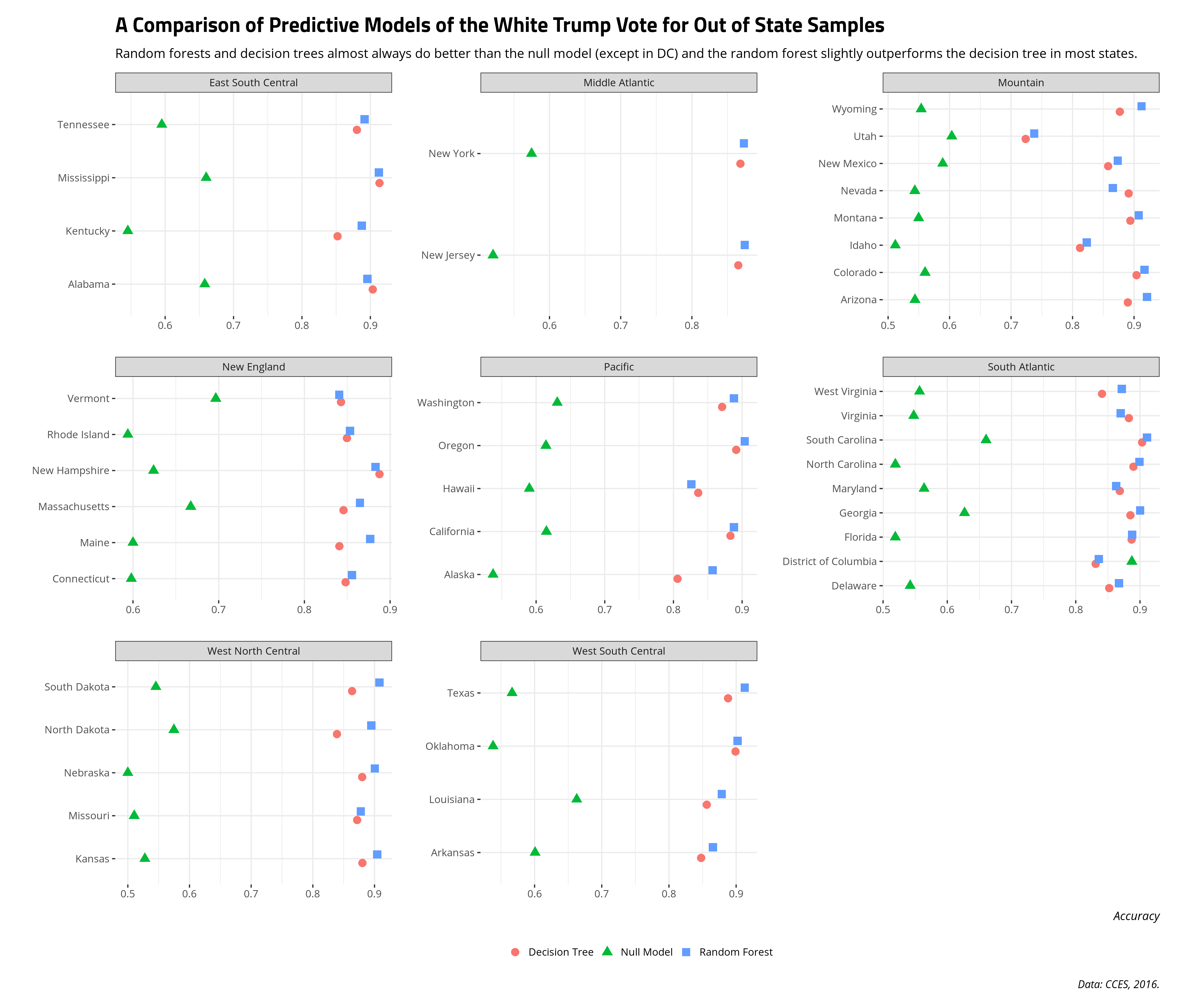
Second, one case stands out where the null model clearly outperforms the random forest model and the decision tree: DC. With only some exaggeration, almost no one voted for Donald Trump in DC (even among white people). If I were to just predict that no one voted for Donald Trump in DC, I would fare better in my predictions than if I were to try to predict the white Trump vote in DC with insights from these various attributes from these select Midwestern states. In my subject domain, we call this a “rare event.” In the machine learning context, this is a “class imbalance” and requires some other considerations about what makes DC unique relative to the other entities in the model (and there is a lot that makes DC unique). Should I revisit this again down the road, I’ll want to consider that imbalance problem and adjust my modeling procedure accordingly. Much like Idaho and Utah, it would also suggest that training a model on white people in states like Ohio and Indiana to predict DC is going to miss some important attributes of white people living in DC.
Conclusion
I wrote this mostly as a guide for myself. I wanted to dig into the world of machine learning a bit more just in case I need to make a career move and if things start heading that far south in academia. In that case, I should demonstrate some familiarity with these tools since they are in high demand in the private sector. They are also not tools we generally learn in the social sciences. In my world, neat causal identification and “explanation” are more important than tools that assist with hypothesis generation and prediction. It’s a false dichotomy—por que no los dos (if you will)—but that’s the way my little world works.
It’s also just a small fraction of stuff to cover and I’ll probably dig into that some other time. I gave no consideration to the optimal number of samples or trees in the random forest context. I gave no consideration to pruning trees that lower the default split threshold. I didn’t mention thinking about prediction error in terms of root mean squared error or mean absolute error. I also left a discussion of ROC curves and the bias-variance trade-off off the table. Those will be topics for another time.
I’ll close with a word of caution about what I did. Namely, I did this just to do it. I started with the idea of doing a simple train/test cross-validation on some select Midwestern states and thought, on the fly, to do some out-of-sample predictions in other states just to see what happens. I used data that were already “pre-canned” because I had done them elsewhere on my blog. A social scientist might object there should be a good reason to think about training on some Midwest states to predict more generally. Accordingly, there are probably some features that could be useful in picking up what I’m missing in DC, Idaho, and Utah. That’s where I think a more social scientific approach is valuable for doing machine learning. Subject domain expertise will give a good intuition to what to consider in doing predictive analytics. In this case, I did this just to do it. It didn’t turn out that bad, but there’s more I could do.
-
There are other uses of machine learning or however you’d like to classify a suite of supervised learning techniques. These include determining what variables are useful inputs, helping generate hypotheses, and just generally understanding how a system works. ↩
-
Don’t get me started on the causal identification crowd, though. ↩
Disqus is great for comments/feedback but I had no idea it came with these gaudy ads.