Summarizing Ordinal Models with Simulation from a Multivariate Normal Distribution

- A sign at a July 7, 2016 protesting the epidemic of unsanctioned police murder targeting black communities in the United States (Karla Ann Cote via Getty Images)
This is a simple add-on to my previous post on how to make the most of your regression model. Part of that post, largely targeted to my grad-level methods class, talked about extracting quantities of interest from the regression model through simulation. I mention a pseudo-Bayesian (or “informal Bayesian”, per Gelman and Hill’s (2007, Chp. 7) language) approach that leans on the multivariate normal distribution. Subject to approximate regularity conditions and sample size, the conditional distribution of a quantity of interest, given the observed data, can be approximated with a multivariate normal distribution with parameters derived from the regression model. These are the betas from the regression model with a variance provided by the variance-covariance matrix. This is a clever approach, even as the pseudo-Bayesian aspect of it means there is no prior distribution on the model parameters. Prior distributions are sine qua non features of Bayesian analysis. Instead, this approach sweeps the importance of prior assumptions under the rug because the dependence of the posterior distribution on prior assumptions disappears with large enough posterior samples. Typically, 1,000 simulations are enough to do the trick.
This approach is well supported for two types of models: 1) linear models and 2) generalized linear models with binary dependent variables. Those are at least the applications with which I’m most familiar and it’s where I’ve seen this approach done the most. I haven’t seen it as often with ordinal models. To be clear, the sim() function in the {arm} package offers support for polr() function in the {MASS} package. However, there is no functionality for ordinal models estimated from the {ordinal} package. This is unfortunate because the ordinal package has the most comprehensive suite of ordinal models and has great support for all sorts of mixed model extensions. The absence of intuitive prediction functions for those mixed ordinal models in the {ordinal} package compounds matters.
I think what I offer here is a reasonable workaround for these limitations while still hewing to how Gelman and Hill (2007) talk about model simulation. I offer this with three caveats. First, I really need to think of a wrapper function for this that can account for the varying levels in the dependent variable. Everything here is hand-coded, but still accessible. Second, I’m going to focus on just simulations of the fixed effects parameters. I think this is reasonable since most quantities of interest a reviewer will want to see in my field (political science) will care just about the fixed effects. Third, and related to the second point, more complicated simulations and predictions including things like random slopes in addition to varying levels of the random effect are probably better done with a fully Bayesian approach. {tidybayes} and {brms} offer great support for these approaches.
Alas, here are two cool things you can do with model simulation for your ordinal models from the {ordinal} package. First, here are the R packages I’ll be using.
library(stevemisc) # my toy R package with various helper functions
library(stevedata) # has the TV16 data.
library(tidyverse) # for everything
library(ordinal) # for ordinal mixed models
library(modelr) # for data_grid
library(knitr) # for tables
library(kableExtra) # for pretty tables
And here’s a table of contents.
- The Data and the Model(s)
- Better Summarize the Uncertainty of the Model Parameters
- Make Posterior Predictions
The Data and the Model(s)
Much like the previous post, I’ll be using a subset of white voters in five Midwestern states shortly after the 2016 presidential election. These five states are Indiana, Michigan, Ohio, Pennsylvania, and Wisconsin. The data ultimately come from the 2016 Cooperative Congressional Election Study (CCES), but are made available as the TV16 data in {stevedata}.
We want an ordinal model in lieu of the binary GLM from the previous post. So, this post will try to explain variation in one of the four racism variables that are included in the data. We’ll focus on the whiteadv question in the data. Herein, a respondent is given a statement of “white people in the U.S. have certain advantages because of the color of their skin.” The respondent’s response to this prompt ranges from 1 (strongly agree) to 5 (strongly disagree). Per Christopher D. DeSante and Candis W. Smith, higher values indicate higher levels of cognitive racism. Conceptually, this is capturing/coding the concept of racism as a respondent’s awareness (or lack thereof) of structural racism and white privilege that have been defining features of American life for centuries.
We’ll propose a simple—and to be clear: not causal—model that regresses this dependent variable on five covariates: the respondent’s age, whether the respondent is a woman, whether the respondent has a college diploma, the household income of the respondent, the respondent’s ideology (L to C, five-point scale), and the respondent’s partisanship (D to R, seven-point scale). We’ll add a random effect for the state, but we won’t unpack it here. Again, I think this approach is better when focused on just the fixed effects.
TV16 %>%
  filter(racef == "White") %>%
  filter(state %in% c("Indiana","Ohio","Pennsylvania","Wisconsin","Michigan")) %>%
  mutate(whiteadvf = ordered(whiteadv)) -> Data


Data %>%
  # r2sd_at() is in {stevemisc}
  r2sd_at(c("age", "famincr","pid7na","ideo","lcograc","lemprac"))  -> Data

M1 <- clmm(whiteadvf ~ z_age + female + collegeed +  z_famincr +
             z_ideo + z_pid7na + (1 | state),
             data=Data)
Here’s a summary via the {knitr} and {kableExtra} packages, done quietly to hide code that is primarily for formatting. Of note: only age and the gender variable are statistically insignificant covariates. Everything here should be unsurprising and straightforward.
| Term | Estimate | Std. Error | z-value | p-value |
|---|---|---|---|---|
| Age | 0.041 | 0.050 | 0.834 | 0.404 |
| Female | -0.014 | 0.047 | -0.291 | 0.771 |
| College Educated | -0.638 | 0.054 | -11.887 | 0.000 |
| Household Income | -0.155 | 0.050 | -3.098 | 0.002 |
| Ideology (L to C) | 1.601 | 0.065 | 24.503 | 0.000 |
| Partisanship (D to R) | 0.928 | 0.060 | 15.351 | 0.000 |
| 1|2 | -1.941 | 0.053 | -36.548 | 0.000 |
| 2|3 | -0.326 | 0.047 | -6.915 | 0.000 |
| 3|4 | 0.625 | 0.047 | 13.194 | 0.000 |
| 4|5 | 1.596 | 0.051 | 31.492 | 0.000 |
Ordinal logistic regression coefficients are chores to interpret, but here’s how you’d take a stab at relaying this model output to the reader. Observe, for example, that the college education coefficient is -.638. That is negative and statistically significant (i.e. the absolute value of the z-value is over 11). Thus, the natural logged odds of observing a 5 versus a 1, 2, 3, or 4 decreases by about -.638 for a one-unit increase in college education (i.e. going from not having a four-year college diploma to having a college diploma). The natural logged odds of observing a 4 versus a 3, 2, or 1 for the same one-unit increase decreases by -.638. These are contingent on the assumptions of the ordinal logistic model (i.e. parallel lines) that I don’t belabor here.
I noted in my grad-level methods lab and seemingly to a sympathetic audience on Twitter that ordinal models are a pain in the ass to both estimate and communicate to a lay audience. If this is the dependent variable you’re handed, they’re more honest than the OLS model even as the latent variable assumption of the ordinal model maps (kinda) well (enough) to what the OLS estimator does. Alas, be prepared to communicate your model graphically, and with quantities of interest, if this is the model you’re running.
Better Summarize the Uncertainty of the Model Parameters
I’ll refer the reader to Chapter 7 of Gelman and Hill (2007) for how the multivariate normal distribution is a novel way of simulating uncertainty regarding the model output from a generalized linear model. I’ll only note here that simulating values from a multivariate normal distribution of the ordinal model requires only the vector of regression coefficients and the variance-covariance matrix of the fitted model. I’ll also reiterate that the simulations we’ll be doing won’t include the random effect. I’m sure I could add it to the coefficient vector if I wanted to do it, but most applications (i.e. most reviewers) don’t care about the random effect because the random effect in the mixed effects model is mostly there to make standard errors for contextual effects (i.e. state-level covariates in a context like this, had I included them) more conservative. I again refer the reader to fully Bayesian solutions with {brms} and {tidybayes} if they wanted to do this.
With that in mind, let’s extract the vector of coefficient estimates, the variance-covariance matrix (omitting the random effect of the state), and get 1,000 simulations from a multivariate normal distribution with these parameters. The {MASS} package has this as the mvrnorm() function, which I ported to {stevemisc} as smvrnorm(). I did this to avoid function clashes with {tidyverse} components.
coefM1 <- coef(M1) # coef
vcovM1 <- vcov(M1) # vcov
vcovM1 <- vcovM1[-nrow(vcovM1), -ncol(vcovM1)] # vcov, sans state random effect

set.seed(8675309) # Jenny, I got your number...
simM1 <- smvrnorm(1000, coefM1, vcovM1) %>% tbl_df() %>% # 1,000 sims, convert matrix to tbl
  mutate(sim = seq(1:1000)) %>% # create simulation identifier
  select(sim, everything()) # make sim column first in the data
From here, you can offer another summary of the uncertainty of the model’s parameters. This code will admittedly be a little convoluted.
 broom::tidy(M1) %>% # tidy up M1 for context
  # z95 comes with stevemisc for precise values coinciding with areas under N(0,1)
  # also, these lwr/upr bounds make less sense for alphas, but we're not going to belabor those.
  mutate(lwr = estimate - p_z(.05)*std.error,
         upr = estimate + p_z(.05)*std.error) %>%
  mutate(category = "Ordinal Logistic Regression Summary") -> tidyM1

simM1 %>% # we're going to name things to match up nicely with the above output
  gather(term, value, everything(), -sim) %>%
  group_by(term) %>%
  summarize(estimate = mean(value),
            `std.error` = sd(value), # you can laugh now at calling this a std.error, but I'm going somewhere with this
            lwr = quantile(value, .025),
            upr = quantile(value, .975)) %>%
  mutate(category = "Model Simulation Summary") %>%
  # this is why i'm standardizing column names...
  bind_rows(tidyM1, .) %>%
  # group_by fill to drop the alphas
  group_by(term) %>%
  fill(coef.type) %>%
  filter(coef.type == "location") %>%
  ungroup() %>%
  mutate(term = fct_recode(term,
                           "Age" = "z_age",
                           "Female" = "female",
                           "College Educated" = "collegeed",
                           "Household Income" = "z_famincr",
                           "Ideology (L to C)" = "z_ideo",
                           "Partisanship (D to R)" = "z_pid7na")) %>%
  mutate(term = fct_rev(fct_inorder(term))) %>%
  # plot..
  ggplot(.,aes(term, estimate, ymin=lwr, ymax=upr,color=category, shape=category)) +
  theme_steve_web() +
  scale_colour_brewer(palette = "Set1") +
  geom_hline(yintercept =  0, linetype="dashed") +
  geom_pointrange(position = position_dodge(width = .5)) + coord_flip()+
  labs(title = "A Mixed Effects Ordinal Logistic Regression on Acknowledging Structural White Privilege",
       x = "", y = "Coefficient (with 95% Intervals)",
       subtitle = "Nothing here is terribly surprising and simulating allows another means to summarize uncertainty around the parameters.",
       shape = "", color="",
       caption = "Data: CCES, 2016. Sample: white respondents residing in IN, MI, OH, PA, and WI. Random effect of state omitted for presentation.\nHigher values = more disagreement with a prompt that proposes whites have had structural advantages due to their skin color.")
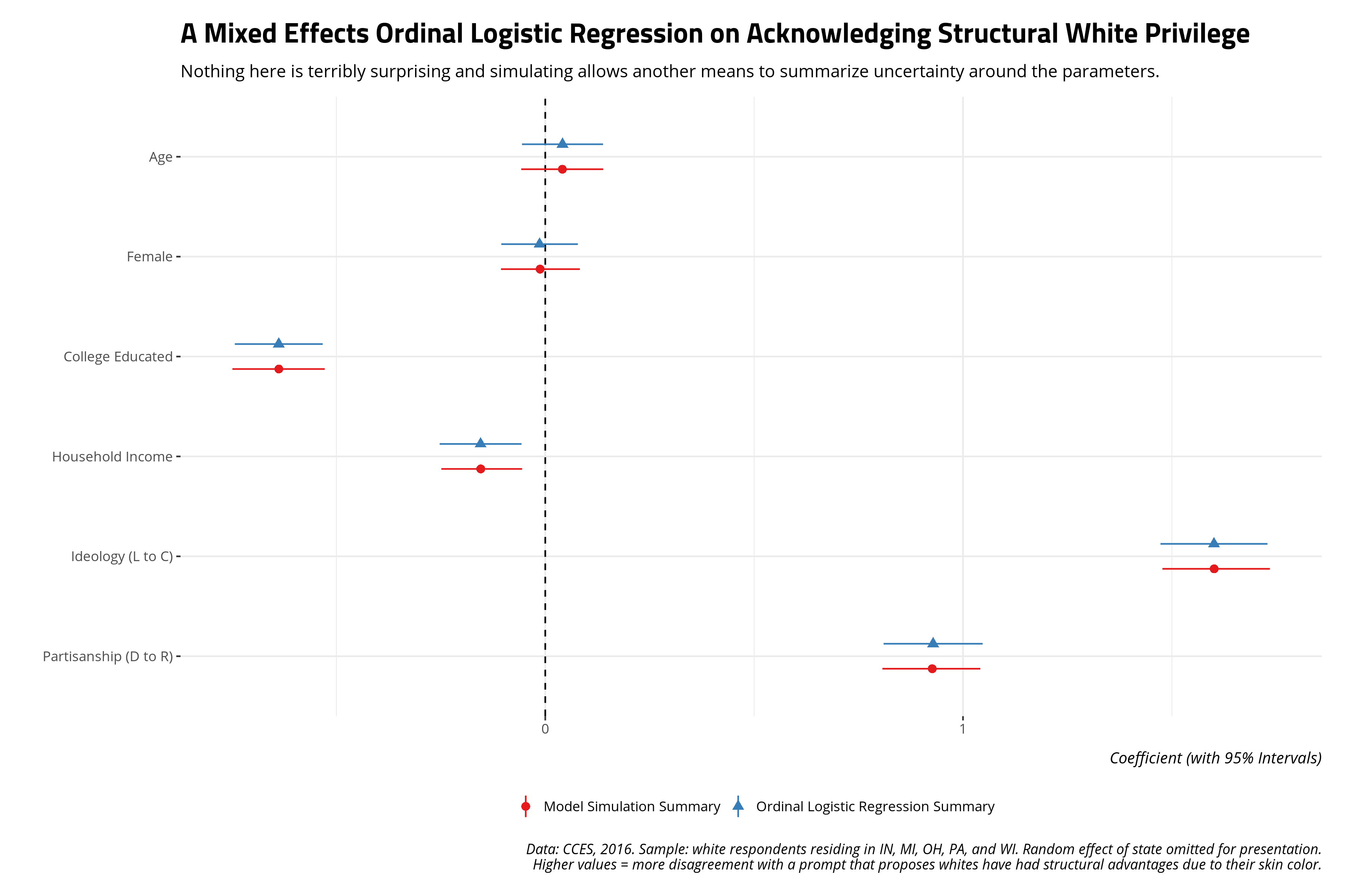
Not a whole lot changes but you can envision situations where interpretations of statistical significance might change under these conditions. This will be a novel way of checking for that from a “pseudo-Bayesian”, or “informally Bayesian”, perspective.
Make Posterior Predictions
I offer this as a potential solution for how to make predictions based on the model output and how to summarize the uncertainty around those predictions without an analytic solution. This had been dogging me for a while. Apparently I’m not the only one, judging from a search of stackoverflow. Here’s how I think you can do this.
First, get 1,000 simulations from a multivariate normal distribution, given the model’s parameters. We already did this and saved the simulations as the simM1 object. Second, get some hypothetical data as a quantity of interest. In my humble opinion, this is critical for anyone estimating and presenting ordinal models. It will be imperative for the researcher to keep things simple and intuitive, given how much goes into an ordinal model. Tailor the quantity of interest to the story you want to tell from your model.
Let’s use the data_grid() function from {modelr} to create two observations that are typical in every way except one. One observation is a person who is very liberal. The other observation is a person who is very conservative. Do note, we’re going to eschew matrix multiplication in R so we’re going to repeat the data a bit.
Data %>%
  # Let's keep it simple and obvious. The min of z_ideo is "very liberal."
  # The max of z_ideo is "very conservative."
  # We should expect to see large magnitude differences.
  data_grid(.model = M1, z_ideo = c(min(z_ideo, na.rm=T), max(z_ideo, na.rm=T))) %>%
  # because we got 1000 sims, we need to repeat this 1000 times
  # ordinal has a slice function that will clash with dplyr
  dplyr::slice(rep(row_number(), 1000)) ->  newdatM1

newdatM1
#> # A tibble: 2,000 × 7
#>    z_ideo  z_age female collegeed z_famincr z_pid7na state
#>     <dbl>  <dbl>  <dbl>     <dbl>     <dbl>    <dbl> <chr>
#>  1 -0.958 0.0518      1         0   0.00220   0.0254 Pennsylvania
#>  2  0.879 0.0518      1         0   0.00220   0.0254 Pennsylvania
#>  3 -0.958 0.0518      1         0   0.00220   0.0254 Pennsylvania
#>  4  0.879 0.0518      1         0   0.00220   0.0254 Pennsylvania
#>  5 -0.958 0.0518      1         0   0.00220   0.0254 Pennsylvania
#>  6  0.879 0.0518      1         0   0.00220   0.0254 Pennsylvania
#>  7 -0.958 0.0518      1         0   0.00220   0.0254 Pennsylvania
#>  8  0.879 0.0518      1         0   0.00220   0.0254 Pennsylvania
#>  9 -0.958 0.0518      1         0   0.00220   0.0254 Pennsylvania
#> 10  0.879 0.0518      1         0   0.00220   0.0254 Pennsylvania
#> # … with 1,990 more rows
Next, we’re going to repeat our simulation data however many unique differences there are in the hypothetical data. In this case, there are only two differences in the hypothetical data (one person is very liberal and the other person is very conservative). So, we’re going to repeat the simulation data twice and arrange it by the simulation number to make sure everything matches up nicely.
simM1 %>%
  # repeat it twice because we have two values of z_ideo
  dplyr::slice(rep(row_number(), 2)) %>%
  # arrange by simulation number after we repeated the data twice
  arrange(sim) -> simM1

simM1
#> # A tibble: 2,000 × 11
#>      sim `1|2`  `2|3` `3|4` `4|5`    z_age  female collegeed z_famincr z_ideo
#>    <int> <dbl>  <dbl> <dbl> <dbl>    <dbl>   <dbl>     <dbl>     <dbl>  <dbl>
#>  1     1 -1.94 -0.315 0.698  1.67  0.0661  -0.0209    -0.567   -0.213    1.61
#>  2     1 -1.94 -0.315 0.698  1.67  0.0661  -0.0209    -0.567   -0.213    1.61
#>  3     2 -1.98 -0.356 0.568  1.60 -0.00399 -0.0663    -0.621   -0.237    1.50
#>  4     2 -1.98 -0.356 0.568  1.60 -0.00399 -0.0663    -0.621   -0.237    1.50
#>  5     3 -1.92 -0.326 0.620  1.63  0.137   -0.0264    -0.559   -0.182    1.56
#>  6     3 -1.92 -0.326 0.620  1.63  0.137   -0.0264    -0.559   -0.182    1.56
#>  7     4 -2.04 -0.401 0.576  1.51  0.0359  -0.0693    -0.778   -0.0638   1.60
#>  8     4 -2.04 -0.401 0.576  1.51  0.0359  -0.0693    -0.778   -0.0638   1.60
#>  9     5 -2.01 -0.395 0.579  1.61 -0.0658  -0.0579    -0.638   -0.187    1.72
#> 10     5 -2.01 -0.395 0.579  1.61 -0.0658  -0.0579    -0.638   -0.187    1.72
#> # … with 1,990 more rows, and 1 more variable: z_pid7na <dbl>
Thereafter, we’re going to rename the columns coinciding with the betas to have a prefix of coef because we’re going to bind_cols() the hypothetical data with it. We don’t want column name clashes and we also want the column names to be a bit clearer and more informative for our own purposes.
simM1 %>%
  # rename these to be clear they're simulated coefficients
  rename_at(vars("z_age", "z_famincr", "z_pid7na", "female", "collegeed", "z_ideo"),
            ~paste0("coef", .)) %>%
  bind_cols(., newdatM1) -> simM1

simM1
#> # A tibble: 2,000 × 18
#>      sim `1|2`  `2|3` `3|4` `4|5` coefz_age coeffemale coefcollegeed
#>    <int> <dbl>  <dbl> <dbl> <dbl>     <dbl>      <dbl>         <dbl>
#>  1     1 -1.94 -0.315 0.698  1.67   0.0661     -0.0209        -0.567
#>  2     1 -1.94 -0.315 0.698  1.67   0.0661     -0.0209        -0.567
#>  3     2 -1.98 -0.356 0.568  1.60  -0.00399    -0.0663        -0.621
#>  4     2 -1.98 -0.356 0.568  1.60  -0.00399    -0.0663        -0.621
#>  5     3 -1.92 -0.326 0.620  1.63   0.137      -0.0264        -0.559
#>  6     3 -1.92 -0.326 0.620  1.63   0.137      -0.0264        -0.559
#>  7     4 -2.04 -0.401 0.576  1.51   0.0359     -0.0693        -0.778
#>  8     4 -2.04 -0.401 0.576  1.51   0.0359     -0.0693        -0.778
#>  9     5 -2.01 -0.395 0.579  1.61  -0.0658     -0.0579        -0.638
#> 10     5 -2.01 -0.395 0.579  1.61  -0.0658     -0.0579        -0.638
#> # … with 1,990 more rows, and 10 more variables: coefz_famincr <dbl>,
#> #   coefz_ideo <dbl>, coefz_pid7na <dbl>, z_ideo <dbl>, z_age <dbl>,
#> #   female <dbl>, collegeed <dbl>, z_famincr <dbl>, z_pid7na <dbl>, state <chr>
This next part will involve manual calculations of the four component of the ordinal logistic regression in M1. First, to reduce redundancy in code, we’ll calculate the estimated value from the design matrix of simulated regression coefficients. Observe how each value of sim appears twice. The coefficients of one of the given 1,000 simulations are identical, as are the hypothetical data except for the one difference (i.e. one person is very liberal and another is very conservative).
simM1 %>%
  mutate(xb = (z_age*coefz_age) + (z_famincr*coefz_famincr) + (z_pid7na*coefz_pid7na) +
                              (female*coeffemale) + (collegeed*coefcollegeed) + (z_ideo*coefz_ideo)) %>%
  select(sim, xb, everything()) -> simM1

simM1
#> # A tibble: 2,000 × 19
#>      sim    xb `1|2`  `2|3` `3|4` `4|5` coefz_age coeffemale coefcollegeed
#>    <int> <dbl> <dbl>  <dbl> <dbl> <dbl>     <dbl>      <dbl>         <dbl>
#>  1     1 -1.54 -1.94 -0.315 0.698  1.67   0.0661     -0.0209        -0.567
#>  2     1  1.43 -1.94 -0.315 0.698  1.67   0.0661     -0.0209        -0.567
#>  3     2 -1.48 -1.98 -0.356 0.568  1.60  -0.00399    -0.0663        -0.621
#>  4     2  1.28 -1.98 -0.356 0.568  1.60  -0.00399    -0.0663        -0.621
#>  5     3 -1.48 -1.92 -0.326 0.620  1.63   0.137      -0.0264        -0.559
#>  6     3  1.37 -1.92 -0.326 0.620  1.63   0.137      -0.0264        -0.559
#>  7     4 -1.58 -2.04 -0.401 0.576  1.51   0.0359     -0.0693        -0.778
#>  8     4  1.36 -2.04 -0.401 0.576  1.51   0.0359     -0.0693        -0.778
#>  9     5 -1.68 -2.01 -0.395 0.579  1.61  -0.0658     -0.0579        -0.638
#> 10     5  1.47 -2.01 -0.395 0.579  1.61  -0.0658     -0.0579        -0.638
#> # … with 1,990 more rows, and 10 more variables: coefz_famincr <dbl>,
#> #   coefz_ideo <dbl>, coefz_pid7na <dbl>, z_ideo <dbl>, z_age <dbl>,
#> #   female <dbl>, collegeed <dbl>, z_famincr <dbl>, z_pid7na <dbl>, state <chr>
Now, we’ll calculate the four logits in the model. Recall, as I made this mistake earlier, most ordinal software packages subtract the design matrix from the particular thetas/alphas. While we’re at it, we’ll convert the logits to probabilities.
simM1 %>%
  mutate(logit1 = `1|2` - xb,
         logit2 = `2|3` - xb,
         logit3 = `3|4` - xb,
         logit4 = `4|5` - xb)  %>%
  mutate_at(vars(contains("logit")), list(p = ~plogis(.))) -> simM1
Finally, we’ll convert those four logit thresholds we just converted to probabilities to get a probability of a given value of the dependent variable.
simM1 %>%
  mutate(p1 = logit1_p,
         p2 = logit2_p - logit1_p,
         p3 = logit3_p - logit2_p,
         p4 = logit4_p - logit3_p,
         p5 = 1 - logit4_p,
         # sump should be 1. Let's check.
         sump = p1 + p2 + p3 + p4 + p5) -> simM1

simM1 %>%
  select(sim, z_ideo, p1:p5, sump)
#> # A tibble: 2,000 × 8
#>      sim z_ideo     p1    p2    p3     p4     p5  sump
#>    <int>  <dbl>  <dbl> <dbl> <dbl>  <dbl>  <dbl> <dbl>
#>  1     1 -0.958 0.401  0.372 0.131 0.0577 0.0387     1
#>  2     1  0.879 0.0334 0.116 0.176 0.236  0.439      1
#>  3     2 -0.958 0.378  0.376 0.131 0.0702 0.0441     1
#>  4     2  0.879 0.0372 0.126 0.166 0.249  0.421      1
#>  5     3 -0.958 0.394  0.367 0.130 0.0662 0.0424     1
#>  6     3  0.879 0.0359 0.119 0.166 0.244  0.436      1
#>  7     4 -0.958 0.387  0.377 0.132 0.0606 0.0435     1
#>  8     4  0.879 0.0324 0.114 0.167 0.225  0.461      1
#>  9     5 -0.958 0.420  0.364 0.122 0.0585 0.0358     1
#> 10     5  0.879 0.0300 0.104 0.157 0.244  0.465      1
#> # … with 1,990 more rows
From there, we can summarize these simulations however we see fit. Let’s summarize these as the mean expected probability with lower and upper bounds defined as a 95% interval around the mean. The magnitude differences between the very liberal and the very conservative become apparent.
simM1 %>%
  mutate(ideo = rep(c("Very Liberal", "Very Conservative"), 1000)) %>%
  select(sim, ideo, p1:p5) %>%
  gather(var, val, -sim, -ideo) %>%
  group_by(ideo, var) %>%
  summarize(mean = mean(val),
            lwr = quantile(val, .025),
            upr = quantile(val, .975)) %>%
  mutate(var = rep(c("Strongly Agree", "Somewhat Agree",
                     "Neither Agree nor Disagree",
                     "Somewhat Disagree", "Strongly Disagree"))) %>%
  mutate_if(is.numeric, ~round(., 3)) %>%
   kable(., format="html", table.attr='id="stevetable"',
         col.names=c("Ideology", "Level of Acknowledgement of White Privilege", "Mean(Probability)", "Lower Bound", "Upper Bound"),
         align = c("l","l","c","c","c"))
| Ideology | Level of Acknowledgement of White Privilege | Mean(Probability) | Lower Bound | Upper Bound |
|---|---|---|---|---|
| Very Conservative | Strongly Agree | 0.034 | 0.029 | 0.039 |
| Very Conservative | Somewhat Agree | 0.115 | 0.103 | 0.129 |
| Very Conservative | Neither Agree nor Disagree | 0.163 | 0.149 | 0.176 |
| Very Conservative | Somewhat Disagree | 0.232 | 0.219 | 0.246 |
| Very Conservative | Strongly Disagree | 0.456 | 0.423 | 0.490 |
| Very Liberal | Strongly Agree | 0.397 | 0.361 | 0.435 |
| Very Liberal | Somewhat Agree | 0.371 | 0.353 | 0.386 |
| Very Liberal | Neither Agree nor Disagree | 0.127 | 0.114 | 0.142 |
| Very Liberal | Somewhat Disagree | 0.062 | 0.054 | 0.072 |
| Very Liberal | Strongly Disagree | 0.043 | 0.036 | 0.049 |
Going forward, I’ll need to think of a way I can automate this with a wrapper function that can be used more generally, but this approach should be generalizable as it is to your particular research question. {ordinal} may not have a lot of built-in prediction support for its mixed models, but simulation through the multivariate normal distribution offers a workaround.
Disqus is great for comments/feedback but I had no idea it came with these gaudy ads.