Replication Forensics

- Admit it; you heard the theme in your head just looking at this image. Peter Thomas is a ringing voice in my head from grad school.
The impetus for this post is as much a concession of defeat as it is a genuine interest of mine. Chatbots have seen enough of my material that they can effectively do my assignments for apathetic students in both my upper-division and lower-division methods courses. I do like the various data sets that I’ve crammed into {stevedata} and spammed onto CRAN. They have real instructional benefits. But, I have to change it up a bit.
Second, I have a genuine interest in the wild, wild west of what was quantitative political science over 20 years ago. Replication norms when I was starting out were nowhere near as rigorous as they are now, but computing power became much cheaper and software options became more sophisticated and user-friendly. It’s crazy to look back on the time when Yale hosted the Journal of Conflict Resolution and had a data repository that has since been lost to history (as far as I’m aware). If you’re lucky, you got a replication data set. If you’re even luckier, the replication data set did not get lost to time when the university underwent one of many structural changes to its web hosting platforms. The replication data set was almost assuredly posted on a faculty member’s website and web hosting platforms at the time were in their infancy. Perhaps, that faculty member may have simply moved the files to something more stable or uploaded them to Dataverse when they retired, switched employers, or had their old web hosting platforms taken from them or rehauled completely. If you’ve won the lottery, that replication data set includes a codebook and a script of some description that allows you to reproduce the findings. It’s led me to do some sleuthing in the furthest reaches of the web to try to find some of these forgotten materials. I have a small but ideally growing Github repository that tries to preserve copies of these data sets that are not easily found and may not even be available on Dataverse.
I also think this is an instructional opportunity for students. We’ve known for some time that replication is necessary for (political) science, and the discipline has since caught up for the most part. But what do you do when all you have is a data set? What do you do when the replication script, if you have one, is in a programming language you’ve never seen before? Well, figure it out.1 In the absence of an exact recipe with software you have, you’ll have to do what I’ll call “replication forensics” to piece together what the author did and how you can translate it to something more current.2 You have the data. You have the article. Figure it out.3
We’re going to do that today with one of my favorite articles I read in graduate school: Kenneth Benoit’s (1996) “Democracies Really Are More Pacific (in General): Reexamining Regime Type and War Involvement”. People reading this who are aware of me know that the bulk of my early research was democratic peace skepticism. I like this article in particular because it tries to tackle one of the biggest contradictions in the democratic peace corpus: the “monadic” phenomenon that is very much implied but never fully confirmed. Benoit (1996), like Rousseau et al. (1996), gives it an honest effort, but the results aren’t terribly convincing the more you look at them. Benoit’s (1996) analysis is also very much limited to a particular moment in time for which there isn’t much assurance that the findings will generalize. That said, it at least acknowledged the tension (which is more than can be said in a lot of democratic peace staples).
Here are the R packages we’ll be using today. I won’t directly load {MASS} but will use it for the negative binomial model function.
library(tidyverse)    # for most things
library(modelsummary) # for regression summary
library(kableExtra)   # for behind-the-scenes formatting
# library(MASS)       # used but not directly loaded.
Reading Benoit (1996)’s Data
I found a copy of Benoit’s (1996) data/analyses and uploaded these files to my pet Github repository for these things. Mercifully, you get a README file that will tell you where to look for replicating certain parts of his analysis. You also get various codebooks (as .cbk files) to assist you. That’s certainly nice, though I will say I didn’t look at them before writing this post and won’t look at them now. Seriously. I’m trying to practice what I preach; “figure it out”.
I want to replicate his Table 2, a screenshot of which follows.
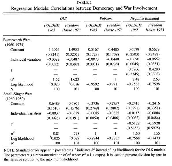
- Table 2 in Benoit (1996)
The README file is pointing me to the WEEDE.ASC file for the data and the REG_TAB2.PRG file to replicate this. I’ll have to use the former but I’m going to avoid the latter for the sake of this exercise. I’ll get to the data shortly, but the reader and I are looking at the contents of these files for the first time. Neither of us, in all likelihood, have used the software that Benoit (1996) used for his analysis: GAUSS. I don’t know when exactly GAUSS fell out of favor in my field, but it was certainly before (and likely long before) I joined the field in 2006. Together, we’ll figure it out.
We’ll have to load the data before doing anything with them. I can already tell from context clues and, well, opening the WEEDE.ASC file in a text editor, that there is going to be a small issue. Here are the column names and the first row of the data file.
@ ccode	cname	superpwr	butterw	kende	ssm_is	ssm_es	ssis6074	sses6074	ssis7580	sses7580	ssal6080	ssal6074	ssal7580	poldem60	poldem65	civil73	polit73	civil79	polit79	fh73	fh75_80	dembin	area	defexd	defexdpc	encon	enconpc	gnppc	gdppc	impexppc	impexp	ecintdep	tvpc	szmil	szmilpc	popltn	larea	lpopltn	lszmil	lszmilpc	ltvpc	lecintd	limpexpc	limpexp	lencnpc	lgdppc	milwp70	popln70	ecnpc70	trade75	lmilwp70	lpopln70	lecnpc70 @
2	United_States	1	7	14	1	0	1	0	0	0	1	1	0	94.6	92.4	1	1	1	1	14	14	1	3619	76276144	37229	2278900	11127	4953	4501	40192	8234600	0.081	41292	3161	154	204880	3.559	5.311	3.5	2.188	4.616	-1.091	4.604	6.916	4.046	3.653	24.2	204879	11077	13.8	1.3838	5.3115	4.0444
That leading @ is going to be a slight frustration because R will want to read that as a column. There are certainly context clues that come with experience, but even the lay reader can see how this will go awry. My knowledge of the Correlates of War state system tells me that the United States has a state code of 2. It should be the case that ccode is the column that has that 2, but R will read a column of @ as having that 2. I don’t want that.
You have one of two options here. The first is to make a copy of the file, erase the @ and save. That’s certainly the easiest way to go about this and it’s what I would advise students to do under these circumstances. You could also do something like this.
Data <- read_file("~/Koofr/data/benoit1996drmp/WEEDE.ASC")
# ^ assuming your data are here, which they won't be. Adjust to taste.

substring(Data, 1, 150) # looks gross, but don't worry
#> [1] "@ ccode\tcname\tsuperpwr\tbutterw\tkende\tssm_is\tssm_es\tssis6074\tsses6074\tssis7580\tsses7580\tssal6080\tssal6074\tssal7580\tpoldem60\tpoldem65\tcivil73\tpolit73\tci"
Data <- gsub("@", "", Data) # find any instance of @ and replace with nothing at all.
Data <- read_table(Data) # read the table

Data # ta-da
#> # A tibble: 101 × 55
#>    ccode cname   superpwr butterw kende ssm_is ssm_es ssis6074 sses6074 ssis7580
#>    <dbl> <chr>      <dbl>   <dbl> <dbl>  <dbl>  <dbl>    <dbl>    <dbl>    <dbl>
#>  1     2 United…        1       7    14      1      0        1        0        0
#>  2    20 Canada         0       0     0      0      0        0        0        0
#>  3    40 Cuba           0       1     2      0      1        0        0        0
#>  4    41 Haiti          0       0     0      0      0        0        0        0
#>  5    42 Domini…        0       1     1      0      0        0        0        0
#>  6    70 Mexico         0       0     0      0      0        0        0        0
#>  7    90 Guatem…        0       0     1      0      0        0        0        0
#>  8    91 Hondur…        0       1     1      1      0        1        0        0
#>  9    92 El_Sal…        0       1     1      1      0        1        0        0
#> 10    93 Nicara…        0       0     0      0      0        0        0        0
#> # ℹ 91 more rows
#> # ℹ 45 more variables: sses7580 <dbl>, ssal6080 <dbl>, ssal6074 <dbl>,
#> #   ssal7580 <dbl>, poldem60 <chr>, poldem65 <chr>, civil73 <dbl>,
#> #   polit73 <dbl>, civil79 <chr>, polit79 <chr>, fh73 <dbl>, fh75_80 <dbl>,
#> #   dembin <dbl>, area <dbl>, defexd <chr>, defexdpc <chr>, encon <dbl>,
#> #   enconpc <dbl>, gnppc <chr>, gdppc <chr>, impexppc <chr>, impexp <chr>,
#> #   ecintdep <chr>, tvpc <chr>, szmil <chr>, szmilpc <chr>, popltn <dbl>, …
An approach like this won’t be necessary if you’re handed a .sav file (SPSS format) or a .dta file (Stata format), but it’s something you’ll want to think about if you have a text file offered as a data file. This may just be a GAUSS quirk for all I know, though flat text files are ubiquitous in older analyses for which data are available. You should learn to anticipate some of these problems. Definitely look before you do anything.
Identifying the Variables in Benoit’s (1996) Table 2
I’ve read Benoit’s (1996) article to know what he is doing. He’s regressing two different measures of war counts (Butterworth and Small-Singer) on two different measures of democracy (Bollen’s (1980) measure of democracy and a measure of democracy from Freedom House). He will do that for three different estimation techniques: the linear model/OLS, the Poisson model for counts, and the negative binomial model (used for over-dispersed/under-dispersed counts). I could look at the program file that accompanies this analysis, but I won’t for the sake of what I encourage students to do for themselves. Figure it out.
Let’s identify the column names in the data if they’ll signal what we want.
colnames(Data)
#>  [1] "ccode"    "cname"    "superpwr" "butterw"  "kende"    "ssm_is"
#>  [7] "ssm_es"   "ssis6074" "sses6074" "ssis7580" "sses7580" "ssal6080"
#> [13] "ssal6074" "ssal7580" "poldem60" "poldem65" "civil73"  "polit73"
#> [19] "civil79"  "polit79"  "fh73"     "fh75_80"  "dembin"   "area"
#> [25] "defexd"   "defexdpc" "encon"    "enconpc"  "gnppc"    "gdppc"
#> [31] "impexppc" "impexp"   "ecintdep" "tvpc"     "szmil"    "szmilpc"
#> [37] "popltn"   "larea"    "lpopltn"  "lszmil"   "lszmilpc" "ltvpc"
#> [43] "lecintd"  "limpexpc" "limpexp"  "lencnpc"  "lgdppc"   "milwp70"
#> [49] "popln70"  "ecnpc70"  "trade75"  "lmilwp70" "lpopln70" "lecnpc70"
#> [55] "X55"
Use your eyes, your head, and the context clues from Table 2. Notice Benoit (1996) says that Butterworth’s (1976) conflict data is one of his dependent variables. We can clearly see a column named butterw, and the only such column with a name that remotely matches the description we want. That tells us that’s our dependent variable. We’ll need a bit more sleuthing to discern what could be the Singer-Small data he’s using. Three context clues are guiding me here. First, it’s usually—not always: usually—the case that the main variables of interest to a researcher are in the first few columns. They’re not typically at the end. So, I’m starting to look at the first few columns I see. The second context clue is ss, suggesting “Singer and Small”. I see a few columns that start with that, which all have numbers following them. There’s my third context clue: they’re signaling the temporal domain of the count of wars. Per Table 2, the temporal domain of these count of wars says they span 1960 to 1980. Putting all those context clues together, I know ssal6080 is my second dependent variable.
I can do something similar for the two measures of democracy that serve as his independent variables. Benoit (1996) helpfully tells you the political democracy measure benchmarks to 1965. My eyes see two columns as potential candidates for this variable: poldem60 and poldem65. Given the information available, it seems like poldem65 is the obvious candidate for what he says is “POLDEM 1965” in his analysis. Following this logic, I can again discern what would be the Freedom House measure from 1973. It should be fh1973, signaling Freedom House’s measure of democracy in 1973. Here would be a reduced version of the data.
Data %>%
  select(ccode:cname, butterw, ssal6080, poldem65, fh73)
#> # A tibble: 101 × 6
#>    ccode cname              butterw ssal6080 poldem65  fh73
#>    <dbl> <chr>                <dbl>    <dbl> <chr>    <dbl>
#>  1     2 United_States            7        1 92.4        14
#>  2    20 Canada                   0        0 99.5        14
#>  3    40 Cuba                     1        1 5.2          2
#>  4    41 Haiti                    0        0 20.7         3
#>  5    42 Dominican_Republic       1        0 38.8        11
#>  6    70 Mexico                   0        0 74.5         8
#>  7    90 Guatemala                0        0 39.5        11
#>  8    91 Honduras                 1        1 50           6
#>  9    92 El_Salvador              1        1 72.1        11
#> 10    93 Nicaragua                0        0 55.4         9
#> # ℹ 91 more rows
Doing this, though, alerted me to a potential issue I’ll want to consider. R read the poldem65 as a character when I know it should be a numeric variable. We’ll have to find out what happened.
Data %>% distinct(poldem65) %>% pull()
#>  [1] "92.4" "99.5" "5.2"  "20.7" "38.8" "74.5" "39.5" "50"   "72.1" "55.4"
#> [11] "90.1" "76.9" "71.4" "73.4" "44.6" "87"   "60.9" "36.2" "44.7" "97"
#> [21] "52.6" "99.6" "99.1" "97.2" "99.7" "99.9" "90.8" "10.4" "39"   "88.6"
#> [31] "18.1" "22.1" "97.1" "11.6" "20.5" "96.8" "18.2" "50.8" "82.8" "37.5"
#> [41] "20.9" "97.3" "37.2" "53.7" "24.7" "16"   "45.6" "37.3" "7.2"  "23.7"
#> [51] "45.5" "56"   "49.5" "34.2" "47.6" "38.5" "77"   "12.5" "58.9" "83"
#> [61] "32.2" "63.6" "34.4" "37.9" "45"   "76.4" "11.4" "38.7" "19.9" "74"
#> [71] "30.8" "9.7"  "6.5"  "23.2" "16.4" "22.8" "21"   "53"   "99.8" "91.2"
#> [81] "62.5" "."    "85.9" "29.2" "17.3" "36.3" "42.8" "33.1" "12.4" "80.3"
#> [91] "92.6" "9.8"  "100"
It looks like the missing data code for this measure is a .. If I knew in advance this was an issue, I could’ve potentially passed it off as an argument in the read_table() function (i.e. read_table(Data, na = ".")). But, I’m only catching this now. We’ll find out what observation this is first before fixing it. We can already deduce from Table 2 that it concerns just one observation.
Data %>%
  select(ccode:cname, butterw, ssal6080, poldem65, fh73) %>%
  filter(poldem65 == ".") # Burma...
#> # A tibble: 1 × 6
#>   ccode cname butterw ssal6080 poldem65  fh73
#>   <dbl> <chr>   <dbl>    <dbl> <chr>    <dbl>
#> 1   775 Burma       0        0 .            4

Data %>% mutate(poldem65 = ifelse(poldem65 == ".", NA, poldem65),
                poldem65 = as.numeric(poldem65)) -> Data

Data %>%
  select(ccode:cname, butterw, ssal6080, poldem65, fh73)
#> # A tibble: 101 × 6
#>    ccode cname              butterw ssal6080 poldem65  fh73
#>    <dbl> <chr>                <dbl>    <dbl>    <dbl> <dbl>
#>  1     2 United_States            7        1     92.4    14
#>  2    20 Canada                   0        0     99.5    14
#>  3    40 Cuba                     1        1      5.2     2
#>  4    41 Haiti                    0        0     20.7     3
#>  5    42 Dominican_Republic       1        0     38.8    11
#>  6    70 Mexico                   0        0     74.5     8
#>  7    90 Guatemala                0        0     39.5    11
#>  8    91 Honduras                 1        1     50       6
#>  9    92 El_Salvador              1        1     72.1    11
#> 10    93 Nicaragua                0        0     55.4     9
#> # ℹ 91 more rows
Cool, let’s proceed.
Replicating Benoit’s (1996) Table 2
There is definitely a convoluted way of making a loop and list of these various models, though it would be beyond the scope of this post to do this and might only serve to overwhelm my students reading this. So, we’ll do it the tedious way. Let’s do the Butterworth wars first.
M1 <- lm(butterw ~ poldem65, Data)
M2 <- lm(butterw ~ fh73, Data)
M3 <- glm(butterw ~ poldem65, Data, family = "poisson")
M4 <- glm(butterw ~ fh73, Data, family = "poisson")
M5 <- MASS::glm.nb(butterw ~ poldem65, Data)
M6 <- MASS::glm.nb(butterw ~ fh73, Data)
A regression table, by way of {modelsummary}, follows.
| POLDEM 1965 (OLS) | FH 1973 (OLS) | POLDEM 1965 (Poisson) | FH 1973 (Poisson) | POLDEM 1965 (NB) | FH 1973 (NB) | |
|---|---|---|---|---|---|---|
| Democracy | −0.0082 | −0.0487 | −0.0073* | −0.0448+ | −0.0071 | −0.0437 |
| (0.0052) | (0.0389) | (0.0031) | (0.0237) | (0.0048) | (0.0363) | |
| Intercept | 1.6026*** | 1.4953*** | 0.5167** | 0.4405* | 0.5068+ | 0.4333 |
| (0.3241) | (0.3205) | (0.1729) | (0.1777) | (0.2841) | (0.2882) | |
| R2 | 0.025 | 0.016 | ||||
| Log.Lik. | −189.074 | −191.188 | −166.703 | −168.858 | −147.559 | −148.649 |
| Num.Obs. | 100 | 101 | 100 | 101 | 100 | 101 |
| + p < 0.1, * p < 0.05, ** p < 0.01, *** p < 0.001 |
By and large, we’ve replicated what Benoit (1996) reports in his Table 2 for the analysis of Butterworth’s war data. It does come with two caveats that are immediately discernible. The first one is an advanced note in which I have to confess that I have no idea how GAUSS is calculating the log likelihood of the Poisson models. I only know of the one way of doing it (i.e. how R does it: sum(dpois(M3$y, lambda = fitted(M3), log = TRUE))). However, that’s an advanced note that I cannot earnestly expect students to know (because I wouldn’t know it myself). More importantly, the coefficients are identical. The same cannot be said about the negative binomial regression. Here, there is some interesting disagreement. I finally peeked into the information that Benoit (1996) makes available. The negative binomial regression in the program file seems like it was custom written for the task at hand. I can already discern the different parameterizations of dispersion, which are also stated in the footnote of the table. I can already see different starting values for the dispersion parameter, or at least I think I do. I know the glm.nb() function in the {MASS} package starts with the Poisson and that doesn’t seem(?) to be where the negative binomial routine starts in GAUSS. To be clear, the differences are rather slight with all that in mind. But, they can’t go unnoticed.
They’re also immaterial for my intended audience. I can’t expect intro-level students to know those advanced details, but I can expect them to dig into the data to discern the basic information and modeling techniques. Toward that end, we’ve accomplished the first half of Table 2.
Now, let’s round home with a replication of the second half of Table 2, where the dependent variable is the Singer and Small wars.
M7 <- lm(ssal6080 ~ poldem65, Data)
M8 <- lm(ssal6080 ~ fh73, Data)
M9 <- glm(ssal6080 ~ poldem65, Data, family = "poisson")
M10 <- glm(ssal6080 ~ fh73, Data, family = "poisson")
M11 <- MASS::glm.nb(ssal6080 ~ poldem65, Data)
M12 <- MASS::glm.nb(ssal6080 ~ fh73, Data)
Summarize it for us, {modelsummary}.
| POLDEM 1965 (OLS) | FH 1973 (OLS) | POLDEM 1965 (Poisson) | FH 1973 (Poisson) | POLDEM 1965 (NB) | FH 1973 (NB) | |
|---|---|---|---|---|---|---|
| Democracy | −0.0037 | −0.0329+ | −0.0085+ | −0.0825* | −0.0083 | −0.0850+ |
| (0.0026) | (0.0191) | (0.0050) | (0.0407) | (0.0061) | (0.0488) | |
| Intercept | 0.6489*** | 0.6801*** | −0.3736 | −0.2757 | −0.3863 | −0.2593 |
| (0.1610) | (0.1576) | (0.2748) | (0.2805) | (0.3535) | (0.3547) | |
| R2 | 0.020 | 0.029 | ||||
| Log.Lik. | −119.136 | −119.526 | −92.150 | −91.824 | −88.752 | −88.501 |
| Num.Obs. | 100 | 101 | 100 | 101 | 100 | 101 |
| + p < 0.1, * p < 0.05, ** p < 0.01, *** p < 0.001 |
The same basic story emerges. We’ve just about perfectly reproduced the linear model output and the Poisson model output (barring the log-likelihood in the latter). There’s also the interesting discrepancy in the negative binomial regression, though we’ll have to chalk that up to different optimization and parameterization procedures that I cannot honestly expect students to know at this point in their studies.
Conclusion
The purpose of this post isn’t to point fingers. I actually rather appreciate that the author had these data available and actually included a full-fledged codebook, script, and output log to show his work. Speaking from experience, that was rather anomalous for scholarship at this time. Further, the point isn’t to further scrutinize democratic peace scholarship anymore than I already have in the bulk of my early published scholarship. This is more of a warning and a sales pitch to my students. I’m going to present something like this to you soon because I think it’s beneficial to your education. You will learn a lot by replication, yes. But, you’ll also learn a lot as well by doing some forensics to figure it out for yourself how others did it in the presence of poorly sourced data. I have an example I’m going to roll out to my Master’s students that will be a bit simpler in presentation, but actually won’t at all have a codebook or other documentation beyond the published article itself.
You’ll just have to figure it out. You’ll learn a lot in the process.
-
One legendary case of this is the scope of work by Herndon et al. (2014) to document the deception and carelessness of Reinhart and Rogoff (2010). You can read my reproduction of Herndon et al.’s (2014) work here. What I’m asking students to do has that same spirit, though ideally not the same ramifications. ↩
-
The use of this term may be somewhat stark because it likens a published article to a crime scene. Alas, from one cynical perspective, that’s maybe fair. ↩
-
No one will pay you any serious amount of money to follow a completely prescribed routine. If that were your task, you are immediately replaceable if the next quarterly report looks lukewarm to shareholders. ↩
Disqus is great for comments/feedback but I had no idea it came with these gaudy ads.