How to Calculate Tau-b (τb) Using Alliance Data in R
- We have Maurice Kendall to thank for this measure, and we have ourselves to blame for using it the way we did.
My continued development of {peacesciencer} led me to finally introduce some functionality for calculating dyadic foreign policy similarity, and I thank Frank Häge for allowing me to use the most recent version of his dyadic foreign policy similarity data for that end. Reading his 2011 Political Analysis article that describes an earlier version of the data reminded me of the great S debates in quantitative peace science when I was in graduate school. In that particular application, Häge is offering a series of better measures for dyadic foreign policy similarity than the common measure at the time: Signorino and Ritter’s (1999) S. However, this measure itself was a purported improvement on another common measure for dyadic foreign policy similarity: Kendall’s Tau-b (τb, if you’re fancy). Kendall’s Tau-b, one of three (if I recall correctly) of his rank correlation coefficients dates to a 1938 publication in Biometrika but its use in conflict studies owes to a 1975 publication in Journal of Conflict Resolution by Bruce Bueno de Mesquita. Its incorporation into EUGene made it a very popular measure of dyadic foreign policy similarity before S supplanted it. Few would recommend thinking of Tau-b as a preferred measure of dyadic foreign policy similarity, but its use will on occasion recur. For example, Horowitz and Stam (2014) use it in their influential study of leaders in conflict.
Still, its modern use is rare and may owe as a legacy to EUGene. Häge (2011) says you shouldn’t use it. Signorino and Ritter (1999) say you shouldn’t use it. But, how might you calculate it? Häge doesn’t include Tau-b in his battery of dyadic foreign policy similarity measures, and with good reason. {peacesciencer} currently doesn’t include support for it, but the thought occurred a future update may want to give this a shot. It required me learning a little bit more about how this measure was calculated/used in quantitative peace science articles. What follows is how I understand this measure to be used in quantitative peace science, with a focus on the Correlates of War alliance data.
What is Kendall’s Tau-b?
Kendall’s Tau-b is one of three rank correlation coefficients, which vary for how they handle ties. Kendall’s Tau-b, in particular, is a correlation coefficient that deals with tied ranks by assuming a value of zero indicates an absence of association. The Tau-b coefficient is defined as follows.
\[\tau_B = \frac{n_c-n_d}{\sqrt{(n_0-n_1)(n_0-n_2)}}\]Where:
\[\begin{align} n_c & = \text{Number of concordant pairs} \\ n_d & = \text{Number of discordant pairs} \\ n_0 & = n(n-1)/2\\ n_1 & = \sum_i t_i (t_i-1)/2 \\ n_2 & = \sum_j u_j (u_j-1)/2 \\ t_i & = \text{Number of tied values in the } i^\text{th} \text{ group of ties for the first quantity} \\ u_j & = \text{Number of tied values in the } j^\text{th} \text{ group of ties for the second quantity} \end{align}\]I can always see this formula, and yet formulas do little to get me to learn something. Indeed, I think that sentiment was shared broadly in political science in the 1990s and early 2000s, so articles on the topic typically offered some toy examples to illustrate what the underlying data might look like to inform these calculations. Consider this reproduction of Table 6 from Signorino and Ritter (1999), which is a comparison of alliance similarity (more on this particular coding later) between Germany and Russia in 1914.
| State | Germany | Russia |
|---|---|---|
| GMY | 3 | 0 |
| RUS | 0 | 3 |
| UKG | 0 | 1 |
| FRN | 0 | 3 |
| AUH | 3 | 0 |
| ITA | 3 | 1 |
| BEL | 0 | 0 |
| SPN | 0 | 0 |
| TUR | 0 | 0 |
| NTH | 0 | 0 |
| SWD | 0 | 0 |
| RUM | 3 | 0 |
| POR | 0 | 0 |
| SWZ | 0 | 0 |
| GRC | 0 | 0 |
| DEN | 0 | 0 |
| YUG | 0 | 0 |
| BUL | 0 | 0 |
| NOR | 0 | 0 |
| ALB | 0 | 0 |
This results in a contingency table, also included in Signorino and Ritter’s (1999) Table 6, in which Germany and Russia share 13 0s (i.e. no alliance contracts for either side). Three German 3s (Germany, Austria-Hungary, and Romania) are all 0s for Russia. One German 3 is a 1 for Russia (Italy). Two Russian 3s are 0s for Germany (Russia, France). From this, Signorino and Ritter calculate a Tau-b for these two in 1914 to be ~.03.
This is when it finally dawned on me that this is all in base R. It’s in the cor() function with an argument I always pass over for Pearson’s r. It’s method = "kendall". Observe.
tribble(~state, ~gmy, ~rus,
        "GMY", 3, 0,
        "RUS", 0, 3,
        "UKG", 0, 1,
        "FRN", 0, 3,
        "AUH", 3, 0,
        "ITA", 3, 1,
        "BEL", 0, 0,
        "SPN", 0, 0,
        "TUR", 0, 0,
        "NTH", 0, 0,
        "SWD", 0, 0,
        "RUM", 3, 0,
        "POR", 0, 0,
        "SWZ", 0, 0,
        "GRC", 0, 0,
        "DEN", 0, 0,
        "YUG", 0, 0,
        "BUL", 0, 0,
        "NOR", 0, 0,
        "ALB", 0, 0) %>%
  summarize(taub = cor(gmy, rus, method="kendall"))
#> # A tibble: 1 × 1
#>     taub
#>    <dbl>
#> 1 0.0303
Well, that’s easy. I’ve could been doing this stuff the whole time in grad school.
How to Create a Dyad-Year Data Set of Tau-b in R
Once you see this for what it is, it doesn’t take too much effort to calculate all this in R. First, here are the packages we’ll need.
library(tidyverse)     # for most things
library(peacesciencer) # for dyad-year and alliance data
library(tictoc)        # for timing stuff
library(foreach)       # for some parallel magic
library(stevemisc)     # for graph formatting
Measures of dyadic foreign policy similarity typically come in two flavors: one uses UN voting data, which are obviously limited to observations after World War II. The other uses the Correlates of War alliance data, which is not as current (most recent year is 2012) but has coverage to 1816. We’re going to use the latter. This is in {peacesciencer} as cow_alliance.
cow_alliance
#> # A tibble: 120,784 × 7
#>    ccode1 ccode2  year cow_defense cow_neutral cow_nonagg cow_entente
#>     <dbl>  <dbl> <dbl>       <dbl>       <dbl>      <dbl>       <dbl>
#>  1      2     20  1949           1           0          1           1
#>  2      2     20  1950           1           0          1           1
#>  3      2     20  1951           1           0          1           1
#>  4      2     20  1952           1           0          1           1
#>  5      2     20  1953           1           0          1           1
#>  6      2     20  1954           1           0          1           1
#>  7      2     20  1955           1           0          1           1
#>  8      2     20  1956           1           0          1           1
#>  9      2     20  1957           1           0          1           1
#> 10      2     20  1958           1           0          1           1
#> # … with 120,774 more rows
What follows is a gigantic caveat since I’ve always hated this train of thought when I was first reading about it in graduate school, even if it never occurred to me how to operationalize Tau-b with the data. Calculating Tau-b like this builds in an assumption that you can construct an ordinal measure of an alliance commitment. The basic train of thought is defense > (neutrality AND/OR non-aggression) > entente > no alliance at all. In their article, Signorino and Ritter (1999) go to great lengths to acknowledge why this is problematic but you should do it anyway. Häge offers the more reasonable take that you should not at all do this and instead use one of his binary measures since you should not think of alliance pledges as ordinal in any way in this typology. {peacesciencer} basically follows Häge’s recommendation and encourages sensible defaults, even if less sensible defaults are available in the data Häge calculated. No matter, we’ll follow what Tau-b calculations were doing at this time and construct an ordinal measure of alliance commitments in the alliance data and grab just what we want.
cow_alliance %>%
  # Create a "commitment" variable
  mutate(commitment = case_when(
    cow_defense == 1 ~ 3,
    cow_defense == 0 & (cow_neutral == 1 | cow_nonagg == 1) ~ 2,
    cow_defense == 0 & cow_neutral == 0 & cow_nonagg == 0 & cow_entente == 1 ~ 1)) %>%
  select(ccode1, ccode2, year, commitment) -> Alliances

Alliances
#> # A tibble: 120,784 × 4
#>    ccode1 ccode2  year commitment
#>     <dbl>  <dbl> <dbl>      <dbl>
#>  1      2     20  1949          3
#>  2      2     20  1950          3
#>  3      2     20  1951          3
#>  4      2     20  1952          3
#>  5      2     20  1953          3
#>  6      2     20  1954          3
#>  7      2     20  1955          3
#>  8      2     20  1956          3
#>  9      2     20  1957          3
#> 10      2     20  1958          3
#> # … with 120,774 more rows
Next, we’ll create a full data set of directed dyad-years from 1816 to 2012 using create_dyadyears() in {peacesciencer}.
DDY <- create_dyadyears(subset_years = c(1816:2012))
DDY
#> # A tibble: 1,760,970 × 3
#>    ccode1 ccode2  year
#>     <dbl>  <dbl> <int>
#>  1      2     20  1920
#>  2      2     20  1921
#>  3      2     20  1922
#>  4      2     20  1923
#>  5      2     20  1924
#>  6      2     20  1925
#>  7      2     20  1926
#>  8      2     20  1927
#>  9      2     20  1928
#> 10      2     20  1929
#> # … with 1,760,960 more rows
Now, we need to draw the rest of the f*cking owl. We’re going to do this in parallel too, using half of our available cores with some assistance from the {foreach} package. For funsies, we’ll use {tictoc} to time this procedure. First, let’s set up {foreach} to do what we want.
# Prepare our cores for work ----

half_cores  <- parallel::detectCores()/2
library(foreach)
my.cluster <- parallel::makeCluster(
  half_cores,
  type = "PSOCK"
)

doParallel::registerDoParallel(cl = half_cores)
foreach::getDoParRegistered()
#> [1] TRUE
Now, it’s owl-drawing time. The following code will create the data we want. I’ll annotate the code with comments to clarify what’s happening.
tic()
Data <- foreach(
  # for each year from 1816 to 2012
  i = 1816:2012
) %dopar% { # disperse across all our available cores, and...
  # subset the alliance data to the given year
  Alliances %>% filter(year == i) -> ally_year
  # subset the dyad-year data to just the given year
  DDY %>% filter(year == i) -> ddy_year

  # Tau-b depends on an assumption states make maximal commitments to defend themselves.
  # So, we need state-v-same-state dyads (e.g. USA-USA-1816) here.
  # That's what this is doing
  ddy_year %>%
    expand(ccode1=ccode1, ccode2=ccode2, year = i) %>%
    # Grab the same-state dyads
    filter(ccode1 == ccode2) %>%
    # Bind 'em
    bind_rows(ddy_year, .) %>%
    # Arrange 'em in order
    arrange(ccode1, ccode2) -> ddy_year

  # Take dyad-year slice of a given year and
  ddy_year %>%
    # merge in what we want
    left_join(., ally_year %>% select(ccode1, ccode2, year, commitment)) %>%
    # Where missing...
    mutate(commitment = case_when(
      # A state makes a maximal commitment to defend itself
      is.na(commitment) & ccode1 == ccode2 ~ 3,
      # A dyad that is not the same state has no alliance
      is.na(commitment) & ccode1 != ccode2 ~ 0,
      TRUE ~ commitment
    )) -> hold_this

  hold_this %>%
    # remove year, we'll get it back later
    select(-year) %>%
    # spread out the data to be more matrix-like
    spread(ccode2, commitment) %>%
    # make it a matrix for easier calculation
    as.matrix() %>%
    # get a correlation matrix of Kendall Tau-b
    cor(method="kendall") %>%
    # Convert back to tibble
    as_tibble() %>%
    # Remove the Tau-bs of ccodes (because you don't want those)
    select(-ccode1) %>% slice(-1) %>%
    # Get new column of unique ccode1s that year
    bind_cols(ddy_year %>% distinct(ccode1), .) %>%
    # take from wide to long
    gather(ccode2, taub, -ccode1) %>%
    # add year identifier
    mutate(year = i) -> hold_this

}
toc() # and, time
#> 84.85 sec elapsed
parallel::stopCluster(cl = my.cluster) # close our clusters
This returned a list of data frames, for each year, of directed dyad-year Tau-bs. All that’s left now is to bind them together into one data frame and remove those same-state dyads that we otherwise needed for the calculation. What emerges is a full directed dyad-year calculation of Tau-b correlation coefficients based on alliance commitments from 1816 to 2012.
Data %>%
  bind_rows(.) %>%
  select(ccode1, ccode2, year, taub) %>%
  filter(ccode1 != ccode2) %>%
  arrange(ccode1, year, ccode2)-> Data

Data
#> # A tibble: 1,761,030 × 4
#>    ccode1 ccode2  year    taub
#>     <dbl> <chr>  <int>   <dbl>
#>  1      2 200     1816 -0.124
#>  2      2 210     1816 -0.0658
#>  3      2 220     1816 -0.0455
#>  4      2 225     1816 -0.0455
#>  5      2 230     1816 -0.0658
#>  6      2 235     1816 -0.0658
#>  7      2 245     1816 -0.156
#>  8      2 255     1816 -0.187
#>  9      2 267     1816 -0.156
#> 10      2 269     1816 -0.156
#> # … with 1,761,020 more rows
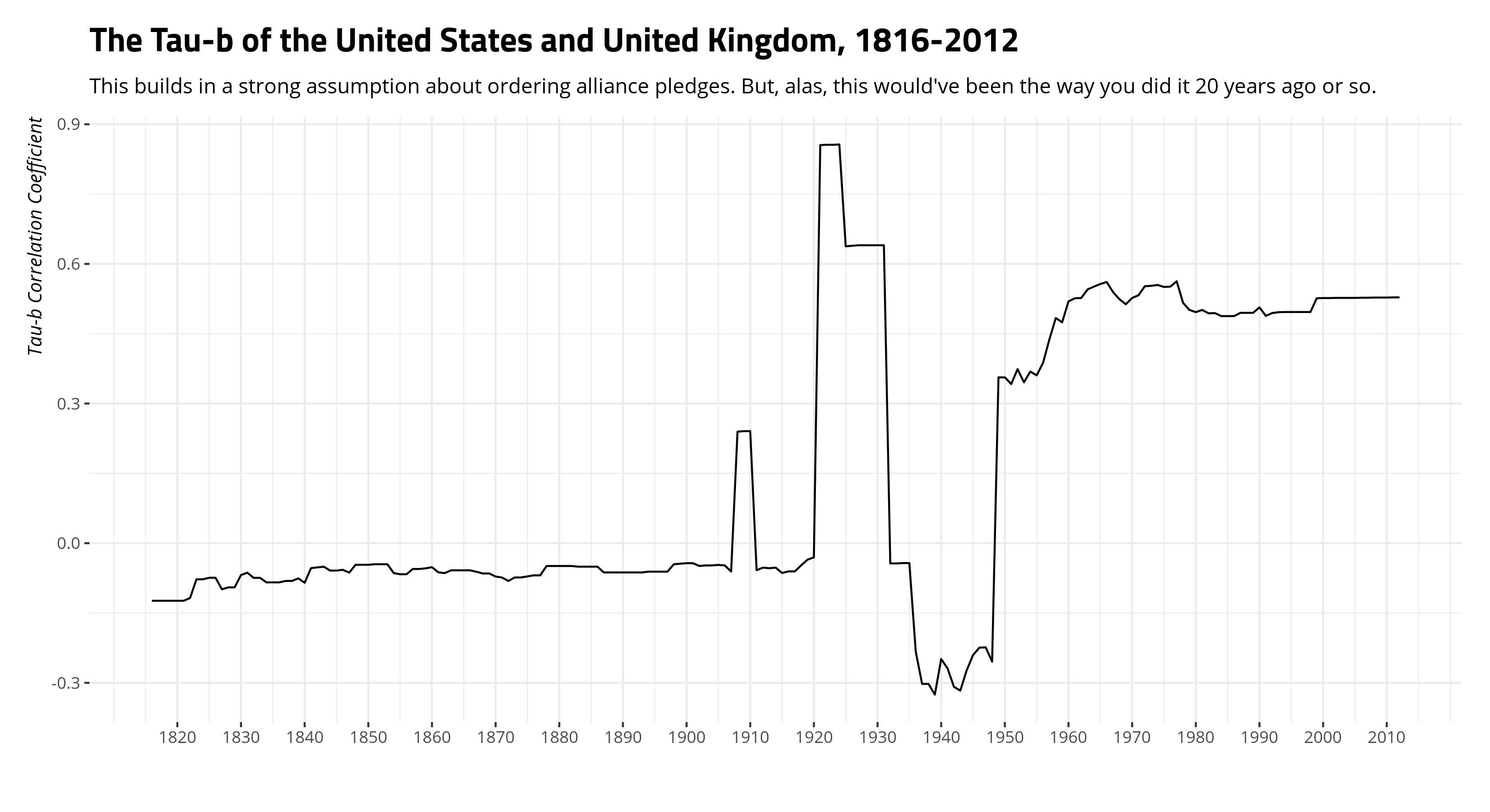
Here, for example, would be the United States and United Kingdom across time.
Data %>%
  filter(ccode1 == 2 & ccode2 == 200) %>%
  ggplot(.,aes(year, taub)) + geom_line() +
  theme_steve_web() +
  scale_x_continuous(breaks = seq(1820, 2010, by = 10)) +
  labs(y = "Tau-b Correlation Coefficient",
       x = "",
       title = "The Tau-b of the United States and United Kingdom, 1816-2012",
       subtitle = "This builds in a strong assumption about ordering alliance pledges. But, alas, this would've been the way you did it 20 years ago or so.")
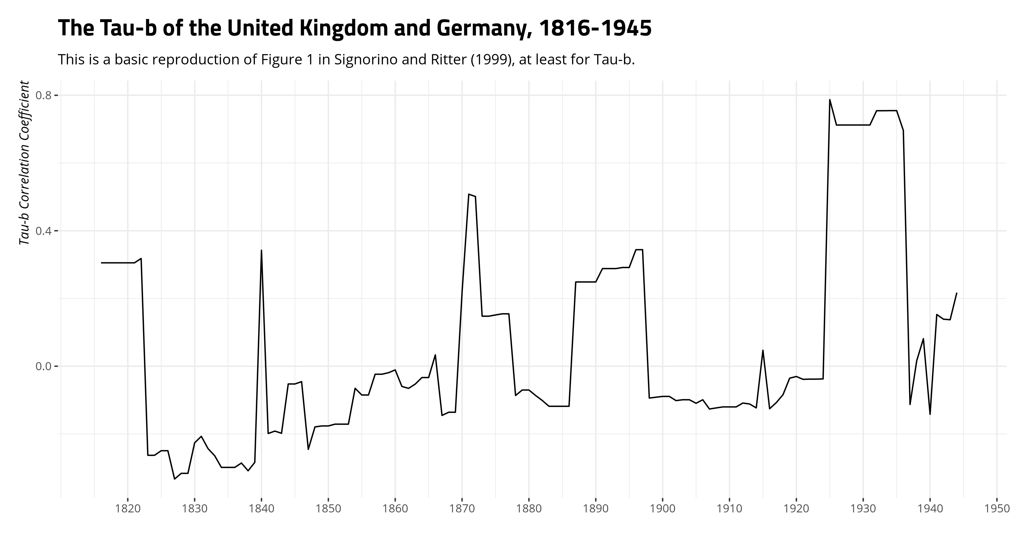
And here would be the United Kingdom and Germany from 1816 to 1945, an effective reproduction of what Signorino and Ritter (1999) report in Figure 1 (albeit with newer data).
Data %>%
    filter(ccode1 == 200 & ccode2 == 255 & year <= 1945) %>%
    ggplot(.,aes(year, taub)) + geom_line() +
    theme_steve_web() +
    scale_x_continuous(breaks = seq(1820, 2010, by = 10)) +
    labs(y = "Tau-b Correlation Coefficient",
         x = "",
         title = "The Tau-b of the United Kingdom and Germany, 1816-1945",
         subtitle = "This is a basic reproduction of Figure 1 in Signorino and Ritter (1999), at least for Tau-b.")
Conclusion
I show how to do this, with a caveat that you should not do this. Tau-b is useful for a lot of things, but not measuring foreign policy similarity by reference to shared alliance portfolios. Toward that end, Signorino and Ritter (1999) are right. Their S doesn’t necessarily capture the concept of dyadic foreign policy similarity either for the reasons that Häge (2011) mentions. His recommendation is Cohen’s (1960) kappa is the best measure for this task, using the binary alliance data.
No matter, here’s how you can do this if, for some reason, you chose to do this.
Disqus is great for comments/feedback but I had no idea it came with these gaudy ads.