Handle Your Academic Projects/Papers in Rstudio with Make and {steveproj}

I write this post as an introduction to an R package under active development, vainly named {steveproj} as part of my suite of eponymous R packages. This package will allow a researcher to start and better maintain an academic project around Make, the R programming language, Rstudio, and some other features of my R ecosystem (prominently: {stevetemplates}). Features of {steveproj} are subject to change while in development but the core of it is, I think, ready to go. While most of what I do is outright navel-gazing or vanity projects, I think this particular project might be publishable in something like Journal of Open Source Software. So, I’ll start first with a discussion of need before elaborating how to use it.
The package is not yet on CRAN, though CRAN is ultimately the goal. Users can install it via my Github.
devtools::install_github("svmiller/steveproj")
The package takes advantage of a Word template I have added to {stevetemplates}, but is not yet on CRAN. The reason for this is simple: CRAN doesn’t like being spammed with package updates and, as of writing, I last updated that package for CRAN about two weeks ago. That forthcoming version— v. 0.5.0—should be on CRAN by early April. Until then, download it via my Github.
devtools::install_github("svmiller/stevetemplates")
Here’s a table of contents.
Statement of Need
Deceptively, some of the largest “costs” that go into any given research project is the maintenance of it in a coherent and accessible way. The causes for this are multiple. For one peer review is a messy and chaotic process. A researcher can devise and implement a neat, simple, and coherent research design on their end, but the end result upon successful publication can look anything like it. If we think of maintaining a research project as akin to curating a garden, the process allows weeds to emerge as the researcher’s project needs to do more than originally intended in order to appease anonymous reviewers. If we think of it as building a car, it’s akin to mounting a laser cannon on top of it. Because.
More downstream weirdness follows when there is no coherent or unified system for manuscript submission. Ideally, an anonymous document is all that is required to initiate a peer review process. However, some journals—and I won’t name names—have their own peculiar standards. A journal might insist that an anonymous document look an exact way, which adds time to a project doing little more than tedious formatting. A journal might insist on having a Word document because it’s always 2003 somewhere. A journal might demand that you upload the LaTeX code and not the LaTeX PDF if that’s what you have, for which, then, it will proudly tell you that it doesn’t have various LaTeX add-ons to compile your PDF for you. The end result here is bogging down the researcher with maintenance issues for a project that was already 99% done.
There already have been major advances on this front. I’ve written and incorporated some of them elsewhere. R Markdown is a wonderful tool for integrating the analyses with the document. You can treat it as an operating system, of a sort, and use it to maintain your projects. What I offer here is an evolution of that approach. This one integrates R Markdown with Make, Rstudio, and some parlor tricks in R and {stevetemplates} to maximize a researcher’s maintenance of their academic project.
Using {steveproj}
The README.md will elaborate this with pictures as well. It also assumes you’ve already installed {steveproj} in R. In Rstudio, go to File > New Project. You’ll see a prompt that looks like this. Select “New Directory”, assuming a new project.

That will direct you here. Scroll here until you see the “S” icon that is incidentally the favicon on my website. Select that entry to create a new academic paper/project.

Thereafter, pick a name—any name—for your project. For clarity’s sake, pick a name that doesn’t have spaces in it since this will be the name of the directory in which you’re working. The Rstudio interface is a wrapper around steveproj::create_project() that will create a new directory with your chosen name and also drop in an .Rproj file to maximize your experience in Rstudio. Rstudio will then immediately kick you into that project.
Alternatively, you could do this through the console in R too.
library(steveproj)
create_project("example-project") # creates new directory in current working directory, titled "example-project"
create_rproj("example-project") # drops an .Rproj into that directory you just created.
The Contents of an Academic Project in {steveproj}
steveproj::create_project() creates a new directory and populates it with the following structure. Assume the directory created was titled “example-project”.
example-project
+-- data
+-- doc
+-- inst
|   +-- refs.bib
+-- R
|   +-- 1-prep.R
|   +-- 2-analysis.R
|   +-- 3-sims.R
+-- src
|   +-- get_citations.R
|   +-- render_docx.R
|   +-- render_pdf.R
|   +-- render_pdf-anon.R
+-- example-project.Rproj
+-- Makefile
+-- ms.Rmd
+-- _output.yaml
+-- README.md
Poking through the contents of the directory and the files within them will make clear what they do, but here’s the intuition of what this setup is designed to do. I’ll discuss it in order of how a research process might unfold. First, the researcher typically collects some data and processes them into various objects, which are then saved (here: in data). Second, the researcher writes about the results in ms.Rmd. Third, the researcher compiles the reports to various documents, which are saved in the doc directory. The researcher maintains responsibility for all components of the project, but Makefile is doing important maintenance and guidance of the process.
Script in R/ and Output to data/
Users are free to monkey with this approach to meet their own needs, but I think the overall advice to embrace a “laundering” approach to reproducible data analyses remains. Researchers should never overwrite raw data. Instead, researchers should write scripts that take raw data, apply various functions to them, and output them to new data objects that are then saved. In this setup, what gets processed in R/ gets saved in data/.
There can be no one-size-fits-all approach to this and what needs to be done will vary by the project type. However, my approach here still leans on Rob Hyndman’s workflow post from 2009 (as it was formative for my development). Generally, social science research I see can be truncated into three objects, around which there are three scripts. I’ll discuss these below.
The first “object” is the main data the researcher will be analyzing. This is processed or “prepped” in this basic setup in R/1-prep.R. Typically, raw data are loaded from somewhere, processed, and saved. This is a minimal working example that leans on these toy data from this post of mine, but observe the intuition from this particular script.
# load libraries ----
# load the functions I need to process the data
library(stevedata) # has the raw data
library(tidyverse) # used for most everything

# "load" the data ----
# Note: in your case, you can load raw data from wherever, even outside the project directory
# For example, if you're analyzing ANES data, you're not ask to stick it in your project directory
# If you can share the raw data, create a directory called "data-raw" in the main project directory
# Then, load it from there.
data(ESS9GB, package="stevedata")

# "prep" the data ----
# I can do anything I want here. I can recode things, transform variables, or whatever
# Here, let's just create a stupid noise variable
set.seed(8675309)
ESS9GB %>%
  mutate(noise = rnorm(nrow(.))) -> Data

# ^ Notice that I "finished" my data prep into a new object, titled "Data"
# Now: I save it to data/Data.rds
saveRDS(Data, "data/Data.rds")
The second object will be the “Model” object. Typically, the researcher runs some set of regressions on the data and stores the output somewhere. In this application, I recommend creating an object, titled Mods, that is a list of however many regressions you run. This will get saved to the data directory as Mods.rds.
Data <- readRDS("data/Data.rds")

Mods <- list()

Mods$"Default" <- lm(immigsent ~ agea + female + eduyrs + uempla + hinctnta + lrscale, data=Data)
Mods$"Default + Noise" <- lm(immigsent ~ agea + female + eduyrs + uempla + hinctnta + lrscale + noise, data=Data)

saveRDS(Mods, "data/Mods.rds")
The third object will be simulations from the model. This could well be unique to political science, but, for the better part of 20 years, political scientists can no longer run a set of regressions, report what was and was not statistically significant, and call it a day. This is the “quantities of interest” movement in which researchers have been implored to communicate quantities of substantive interest along with reasonable estimates of uncertainty. There are, to be clear, any number of ways of doing this, but this movement also came with a renewed interest in “informal Bayesian” approaches to generating these quantities of interest along with estimates of uncertainty.
This sounds daunting, but it just really involves some parlor tricks with a multivariate normal distribution, the vector of model coefficients, and the variance-covariance matrix of the regression model. I have some helper functions for this in {stevemisc}, as you can see below. Assume I wanted to know what changing ideology on a left-right scale does to estimated immigration sentiment in my model. Here’s how I’d go about generating those quantities of interest.
# Libraries first
library(stevemisc)
library(tidyverse)
library(modelr)

# Load stuff
Mods <- readRDS("data/Mods.rds")
Data <- readRDS("data/Data.rds")

Data %>%
  data_grid(lrscale = unique(lrscale), .model = Mods[[1]],
            immigsent = 0) %>% na.omit -> newdat

Sims <- list()

newdat %>%
  # repeat this data frame how many times we did simulations
  dplyr::slice(rep(row_number(), 1000)) %>%
  bind_cols(get_sims(Mods[[1]], newdata = newdat, 1000, 8675309), .) -> Sims$"SQI (Ideology)"

saveRDS(Sims, "data/Sims.rds")
This will conclude the research design section of the academic project. There are three objects I want—a finished data object, a regression model object, and a simulations object. I devise three scripts to produce those, each depending on the other. I process them in R/ to save the output in data/.
Write Your Results in ms.Rmd
The next step is to write about the results in a manuscript. This is done through R Markdown in the ms.Rmd file. {steveproj} comes with a sample R Markdown document to get you started. Here would be the contents of the YAML, which contain important parameters to be processed. I’m assuming some familiarity with R Markdown and YAML but I want to highlight a few things that are unique here. The core of this YAML comes by way of my second article template.
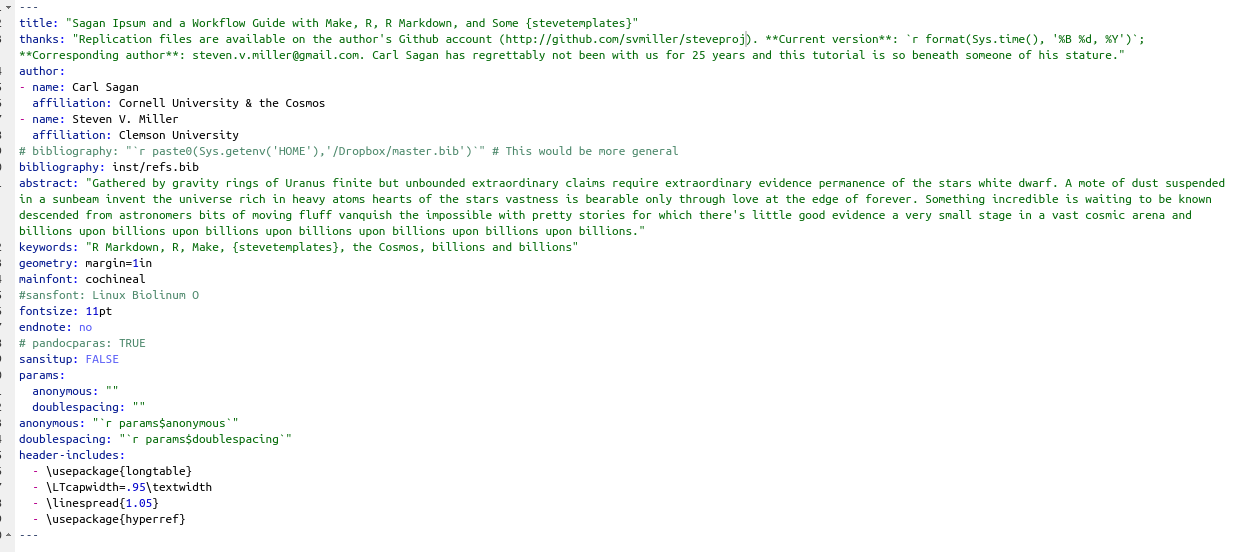
- The YAML of a default {steveproj} ms.Rmd file.
First, notice there is no output specified here. For that reason, if you click the “Knit” button in Rstudio, it will default to HTML. And, for that reason, it’s why {steveproj} comes with the _output.yaml file that disables that button in this project. I thank Andrew Heiss for pointing me toward this hack.
Notice the bibliography: line. For my own cases, I have a master.bib file in my root Dropbox directory that contains everything I’ve ever felt the need to add to it since about 2008. For collaborative projects, perhaps a user may want a shared bibliography file for citations. That appears in the inst/ directory as refs.bib. Later, I’ll show functionality within {steveproj} can farm the ms.Rmd file for citations from a .bib file, even one outside the project directory, and save the citations in a new file in the project directory. For now, I provide the user the option to toggle with this. Certainly, I needed the refs.bib file in the project directory for any user to be able to make this process work.
Finally, I specify a few params entries. These are for anonymizing a PDF for submission. I explain this in the next section.
The ms.Rmd file also comes with this “setup” chunk. You can see what it’s doing here.
# knitr options, mostly for suppressing messages,
# renaming figures and cache
knitr::opts_chunk$set(echo = FALSE,
                      message=FALSE, warning=FALSE,
                      fig.path='doc/figs/',
                      cache.path = 'doc/_cache/',
                      fig.width = 8.5,
                      fig.process = function(x) {
                      x2 = sub('-\\d+([.][a-z]+)$', '\\1', x)
                      if (file.rename(x, x2)) x2 else x
                      })

# Load what you need, and this will be about all you need
library(tidyverse) # for most things
library(stevemisc) # for my default theme
library(modelsummary) # for regression model summaries
library(huxtable) # for formatting tables in Word
library(kableExtra) # for formatting tables in LaTeX

# load the three objects you created
# Note: flexible to whatever you stuck in there.

allrds <- list.files(pattern = ".rds", path = "data") %>%
  stringr::str_remove(., ".rds")

for(i in allrds) {
      filepath <- file.path(paste0("data/",i,".rds"))
      assign(i, readRDS(filepath))
    }

# for conditional evaluation
is_docx <- knitr::opts_knit$get("rmarkdown.pandoc.to") == 'docx'
is_latex <- knitr::opts_knit$get("rmarkdown.pandoc.to") == 'latex'
While I acknowledge it is a little ambitious to treat the R Markdown manuscript file as an operating system for a research project, it does have some incredible properties that you can leverage. Basically, you can lean on R Markdown to write your document AND conditionally evaluate some things based on the desired output. I think there are three main places where you’ll use this: the creation of hypotheses, the production of a regression table, and the creation of a figure.
This is less of an R Markdown hack and more of a Word limitation hack, but Microsoft Word will ignore any LaTeX fields it sees because it won’t know what to do with them. Thus, you can conditionally write hypotheses in LaTeX using LaTeX code while writing a hypothesis as an R Markdown chunk for conditional evaluation (provided the output is to Microsoft Word).
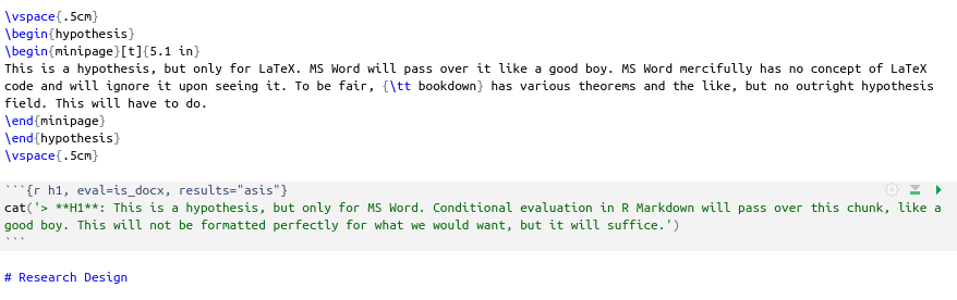
- Conditionally Write Hypotheses in R Markdown
For regression tables, you can employ a three-pronged approach. {modelsummary} is doing most of the heavy-lifting here, but, as of writing, you’ll have to pretty up a regression table in LaTeX differently than you would Word. For LaTeX, it’s {kableExtra}. For Word, it’d be either {huxtable} or {flextable}. Pick you poison of those two. The conditional evaluation would look like this. First, create a minimal regression table in {modelsummary}. If you weren’t going to pretty up it any way, you could stop here.
table_format <- ifelse(is_docx, "huxtable", 'default')

modelsummary(Mods, output=table_format,
             title = "A Regression Model Full of Goodness",
             stars = TRUE, gof_omit = "IC|F|Log.|R2$",
             coef_map = c("agea" = "Age",
                          "female" = "Female",
                          "eduyrs" = "Education (in Years)",
                          "uempla" = "Unemployed",
                          "hinctnta" = "Household Income (Deciles)",
                          "lrscale" = "Ideology (L to R)",
                          "noise" = "Stupid Noise Variable",
                          "(Intercept)" = "Intercept"),
             align=c("lcc")) -> tab_reg
If you wanted to pretty it up in any way, you could do conditional evaluation in R Markdown. Something like this would work.
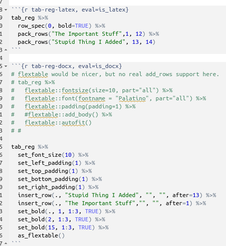
- Conditionally Format Tables in R Markdown
Figures are much less problematic. You could plausibly have just one chunk here instead of three. I’ll only add that, from my limited experience knitting documents to Word, the image quality in Word is way worse than default PDFs in LaTeX. Thus, you might want a conditional graph chunk for Word just to force a higher resolution image. Here’s what it would look like in my sample document.
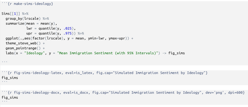
- Conditionally Format Graphs in R Markdown
Those tricks notwithstanding, ms.Rmd is where you report to the outside world what exactly you did as it relates to the research question at hand.
Make Everything with Make
Perhaps the most important part of a {steveproj} academic project is the Makefile. Here are its contents.
# Specify a vew variables to avoid repitition downstream

OUTPUTS=doc/ms.pdf doc/ms-anon.pdf doc/ms.docx
RDS= data/Sims.rds data/Mods.rds data/Data.rds

# Specify the primary targets: the outputs
# Also have a clean option for testing

all: $(OUTPUTS)
refs: inst/refs.bib

clean:
	rm -f $(OUTPUTS) $(RDS)

# Specialty sourcing for each output

doc/ms.pdf:	ms.Rmd $(RDS)
	Rscript -e 'source("src/render_pdf.R")'

doc/ms-anon.pdf: ms.Rmd $(RDS)
	Rscript -e 'source("src/render_pdf-anon.R")'

doc/ms.docx: ms.Rmd $(RDS)
	Rscript -e 'source("src/render_docx.R")'

inst/refs.bib: ms.Rmd
	Rscript -e 'source("src/get_citations.R")'

# Specify what to do for each target .rds

data/Sims.rds: data/Mods.rds R/3-sims.R
	Rscript -e 'source("R/3-sims.R")'

data/Mods.rds: data/Data.rds R/2-analysis.R
	Rscript -e 'source("R/2-analysis.R")'

data/Data.rds: R/1-prep.R
	Rscript -e 'source("R/1-prep.R")'
Someone more sophisticated with Make might scoff at my rudimentary set up, but I think this is both usable and flexible to do various things. Briefly, a Makefile contains a set of recipes that have various targets and dependencies. For each target, if the specified dependency is “newer” than the target (or if the target does not yet exist), the Makefile executes a command.
In this setup, the primary targets are three documents in the doc/ directory. These are doc/ms.pdf (the main LaTeX PDF), doc/ms-anon.pdf (an anonymized PDF), and doc/ms.docx (a Word version of the document). In this setup, the Word document serves just one purpose: it’s there in case any journal insists on having it and not a PDF. If you’ve paid careful attention to how my approach to handling authors in YAML differs from standard R Markdown, you’ll notice that Word’s built-in limitations mean it would not know what to do with it. Thus, the Word version of the manuscript will effectively always be anonymous (unless the researcher chooses to out themselves in the body of the text). It’s not there to be a finished product. It’s there just in case a journal demands to see it.
In Rstudio, you’ll notice there’s a terminal tab right next to the console. If you are in the current working directory of your (Steve) project with this Makefile, enter the following command
make all
That one command will identify the three primary targets—the three documents—and run three separate scripts to create them all. Those scripts are in the src/ directory and can be tweaked to the user’s discretion (e.g. perhaps you want to force keep_tex: TRUE). There is an implicit dependency of ms.Rmd on the three objects created in the R/ scripts. However, those objects are also specified with dependencies. It will create those too. This simple Makefile, just under 40 lines of code in total, manages your project.
I did want to draw attention to one odd-ball target there: inst/refs.bib. I wrote this for those cases where a journal wants your .bib file too even if your master .bib file is outside the project directory. If you want it, run this command:
make inst/refs.bib
That command points to src/get_citations.R. It will farm the ms.Rmd file and identify every citation in the document. It will then match it to the entries in your master .bib file and save it as a new .bib file in the project directory. All it really needs is {stringr} and {bib2df} to do this.
You can download {steveproj} on my Github to get started. I think I want to float this by Journal of Open Source Software to see if there’s interest. It would mean I’d have to do some unit tests. I’m open for feedback as well.
Disqus is great for comments/feedback but I had no idea it came with these gaudy ads.