A Quick Tutorial on Merging Data with the *_join() Family of Functions in {dplyr}

: It's not technically SQL, but it is in spirit.

My graduate studies program director asked me to teach an independent study for a graduate student this semester. The goal is to better train the student for their research agenda beyond what I could plausibly teach them in a given semester.¹ Toward that end, I’m going to offer most (if not all) of the independent study sessions as posts on my blog. This should help the student and possibly help others who stumble onto my website. Going forward, I’m probably just going to copy-paste this introduction for future posts for this independent study.

The particular student is pursuing a research program in international political economy. Substantively, much of what they want to do is outside my wheelhouse. However, I can offer some things to help the student with their research. The first lesson was a tutorial on various state (country) classification systems. This tutorial will be about merging data with the *_join() family of functions available in {dplyr}.

Here’s a table of contents for what follows.

The Issue: No Real Project Has All-Inclusive Data
Relevant R Packages and Data
Mutating Joins
Filtering Joins
My Advice: Get Your Keys Ready Beforehand and Think “Left-Handed”

The Issue: No Real Project Has All-Inclusive Data

The major issue my student is going to encounter is the probability of doing a research project where the data are all-inclusive and self-contained in a single file is almost 0. A reader may object that surveys or survey experiments administered online typically return files that include all the data of importance. That’s fine, but 1) few outside a major survey research organization (e.g. ANES, LAPOP) can get away with doing a simple survey analysis and getting it published at a high-ranking journal in political science, 2) survey experiments cost money that we don’t have (certainly in this economy and at this university), and 3) my student is working in the context of international political economy for which surveys/experiments are not applicable for the desired task. On the last point, my student will likely be having to collect data from the World Bank, the International Monetary Fund, and the Bank of International Settlements. They’ll have to merge all that into one data frame for the sake of an analysis.

I offer this as a guide to the student on the *_join() family of functions that come in {dplyr}. The terminology in these functions seems very much inspired by SQL; indeed, a lot of tidyverse functions have clear corollaries/inspirations in SQL. The functions here are multiple for different purposes, but ultimately merge information from one data set into another based on matching characteristics. The tutorial I offer here will focus on two groups of *_join() functions. The first—mutating joins—adds columns from one data frame to another based on matching rows based on keys. The second—filtering joins—filters rows from one data frame based on the presence or absence of a match in another data frame.

Before getting into the various *_join() functions, I’m going to start with a description of the R packages/data I’ll be using for what follows.

Relevant R Packages and Data

library(tidyverse) # for all things workflow (includes dplyr)
library(stevedata) # for pwt_sample
library(pwt9) # for Penn World Table (9.1) data.

{tidyverse} has most (if not all) of {dplyr}’s functionality, so I opt to load it rather than load just {dplyr}. The other two packages contain the data we’ll be using for this exercise.

First, pwt_sample is a toy data frame I use for various instructional purposes (i.e. about grouping and skew in cross-sectional data). It’s some demographic/macroeconomic data for 21 select (rich) countries based on version 9.1 of the Penn World Table. The data are minimal, including just the country name (country), the country’s three-character ISO code (isocode), the year of the observation (year), the population in millions (pop), the index of human capital per person, based on years of schooling and returns to education (hc), the real GDP at constant 2011 national prices in million 2011 USD (rgdpna), and the share of labor compensation in GDP at current national prices (labsh). The countries included are Australia, Austria, Belgium, Canada, Chile, Denmark, Finland, France, Germany, Greece, Iceland, Ireland, Italy, Japan, Netherlands, Portugal, Spain, Sweden, Switzerland, United Kingdom, and United States of America.

{pwt9} includes the whole Penn World Table data (version 9.1). I’m going to grab just a few columns from these data, but nevertheless keep all countries and years. The variables we’ll grab are the three-character ISO code (isocode), the year of observation (year), the average depreciation rate of the capital stock (delta), and the exchange ration (national currency/USD) (xr).

pwt9.1 %>% as_tibble() %>%
  select(isocode, year,  delta, xr) -> PWT

Here’s the tibble for pwt_sample.

pwt_sample
#> # A tibble: 1,428 x 7
#>    country   isocode  year   pop    hc  rgdpna labsh
#>    <chr>     <chr>   <dbl> <dbl> <dbl>   <dbl> <dbl>
#>  1 Australia AUS      1950  8.39  2.67 119510. 0.680
#>  2 Australia AUS      1951  8.63  2.67 122550. 0.680
#>  3 Australia AUS      1952  8.82  2.68 117534. 0.680
#>  4 Australia AUS      1953  8.99  2.69 130285. 0.680
#>  5 Australia AUS      1954  9.19  2.70 140700. 0.680
#>  6 Australia AUS      1955  9.41  2.70 146250. 0.680
#>  7 Australia AUS      1956  9.64  2.71 146586. 0.680
#>  8 Australia AUS      1957  9.85  2.72 149796. 0.680
#>  9 Australia AUS      1958 10.1   2.73 159957. 0.680
#> 10 Australia AUS      1959 10.3   2.74 169756. 0.680
#> # … with 1,418 more rows

And here’s the tibble for PWT.

PWT
#> # A tibble: 12,376 x 4
#>    isocode  year delta    xr
#>    <fct>   <dbl> <dbl> <dbl>
#>  1 ABW      1950    NA    NA
#>  2 ABW      1951    NA    NA
#>  3 ABW      1952    NA    NA
#>  4 ABW      1953    NA    NA
#>  5 ABW      1954    NA    NA
#>  6 ABW      1955    NA    NA
#>  7 ABW      1956    NA    NA
#>  8 ABW      1957    NA    NA
#>  9 ABW      1958    NA    NA
#> 10 ABW      1959    NA    NA
#> # … with 12,366 more rows

Here’s a breakdown of the two data frames. The temporal domains are identical but the number of countries are not. PWT will have all the countries and years whereas pwt_sample has just 21 select rich countries. Both PWT and pwt_sample have common columns for the country (isocode) and year of observation (year). Both have different economic information (i.e. the columns for real GDP, population, depreciation rate of capital stock, etc.).

Select Territorial Units and Their Various Codes
	PWT	pwt_sample
Number of Countries	182	21
Range of Years	1950:2017	1950:2017
Number of Observations	12,376	1,428
Common Columns	isocode`, `year

Mutating Joins

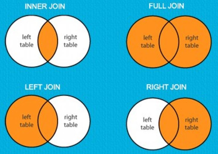
Mutating joins in {dplyr} add columns from one data frames to another based on matching rows on the shared columns. You can think of these matching rows/columns as “keys” or “join predicates.” These joins are as follow.

`inner_join()`

inner_join() includes all rows that appear in both the first data frame (x) and the second data frame (y). Assuming (going forward) that PWT will be the x and pwt_sample will be the y, we’ll do something like this.

inner_join(PWT, pwt_sample)
#> # A tibble: 1,428 x 9
#>    isocode  year  delta    xr country     pop    hc  rgdpna labsh
#>    <chr>   <dbl>  <dbl> <dbl> <chr>     <dbl> <dbl>   <dbl> <dbl>
#>  1 AUS      1950 0.0287 0.893 Australia  8.39  2.67 119510. 0.680
#>  2 AUS      1951 0.0301 0.893 Australia  8.63  2.67 122550. 0.680
#>  3 AUS      1952 0.0310 0.893 Australia  8.82  2.68 117534. 0.680
#>  4 AUS      1953 0.0312 0.893 Australia  8.99  2.69 130285. 0.680
#>  5 AUS      1954 0.0318 0.893 Australia  9.19  2.70 140700. 0.680
#>  6 AUS      1955 0.0325 0.893 Australia  9.41  2.70 146250. 0.680
#>  7 AUS      1956 0.0329 0.893 Australia  9.64  2.71 146586. 0.680
#>  8 AUS      1957 0.0331 0.893 Australia  9.85  2.72 149796. 0.680
#>  9 AUS      1958 0.0334 0.893 Australia 10.1   2.73 159957. 0.680
#> 10 AUS      1959 0.0338 0.893 Australia 10.3   2.74 169756. 0.680
#> # … with 1,418 more rows

In this case, inner_join() returned a data frame the dimension with the number of rows in pwt_sample. It has the effect of adding delta and xr to pwt_sample. inner_join(PWT, pwt_sample) is functionally equivalent to inner_join(pwt_sample, PWT). The ordering of x and y will only affect the order in which the columns appear.

`left_join()`

left_join() returns all rows from x (here: PWT) based on matching rows on shared columns in y (here: pwt_sample). Notice the number of rows equals the number of rows in PWT. The effect is basically adding the economic data from pwt_sample into PWT, if just for the 21 select rich countries included in pwt_sample.

left_join(PWT, pwt_sample)
#> # A tibble: 12,376 x 9
#>    isocode  year delta    xr country   pop    hc rgdpna labsh
#>    <chr>   <dbl> <dbl> <dbl> <chr>   <dbl> <dbl>  <dbl> <dbl>
#>  1 ABW      1950    NA    NA <NA>       NA    NA     NA    NA
#>  2 ABW      1951    NA    NA <NA>       NA    NA     NA    NA
#>  3 ABW      1952    NA    NA <NA>       NA    NA     NA    NA
#>  4 ABW      1953    NA    NA <NA>       NA    NA     NA    NA
#>  5 ABW      1954    NA    NA <NA>       NA    NA     NA    NA
#>  6 ABW      1955    NA    NA <NA>       NA    NA     NA    NA
#>  7 ABW      1956    NA    NA <NA>       NA    NA     NA    NA
#>  8 ABW      1957    NA    NA <NA>       NA    NA     NA    NA
#>  9 ABW      1958    NA    NA <NA>       NA    NA     NA    NA
#> 10 ABW      1959    NA    NA <NA>       NA    NA     NA    NA
#> # … with 12,366 more rows

`right_join()`

right_join() is the companion to left_join(), but returns all rows included in y based on matching rows on shared columns in x (here: PWT). The effect is basically adding the economic data from PWT into pwt_sample, if just for the 21 select rich countries included in pwt_sample.

right_join(PWT, pwt_sample)
#> # A tibble: 1,428 x 9
#>    isocode  year  delta    xr country     pop    hc  rgdpna labsh
#>    <chr>   <dbl>  <dbl> <dbl> <chr>     <dbl> <dbl>   <dbl> <dbl>
#>  1 AUS      1950 0.0287 0.893 Australia  8.39  2.67 119510. 0.680
#>  2 AUS      1951 0.0301 0.893 Australia  8.63  2.67 122550. 0.680
#>  3 AUS      1952 0.0310 0.893 Australia  8.82  2.68 117534. 0.680
#>  4 AUS      1953 0.0312 0.893 Australia  8.99  2.69 130285. 0.680
#>  5 AUS      1954 0.0318 0.893 Australia  9.19  2.70 140700. 0.680
#>  6 AUS      1955 0.0325 0.893 Australia  9.41  2.70 146250. 0.680
#>  7 AUS      1956 0.0329 0.893 Australia  9.64  2.71 146586. 0.680
#>  8 AUS      1957 0.0331 0.893 Australia  9.85  2.72 149796. 0.680
#>  9 AUS      1958 0.0334 0.893 Australia 10.1   2.73 159957. 0.680
#> 10 AUS      1959 0.0338 0.893 Australia 10.3   2.74 169756. 0.680
#> # … with 1,418 more rows

`full_join()`

full_join() includes all rows in x or y. In a case like this, full_join() is ambivalent on what is x and what is y. The choice of x and y will affect the order in which the data are presented back to the user, but not the underlying information

full_join(PWT, pwt_sample)
#> # A tibble: 12,376 x 9
#>    isocode  year delta    xr country   pop    hc rgdpna labsh
#>    <chr>   <dbl> <dbl> <dbl> <chr>   <dbl> <dbl>  <dbl> <dbl>
#>  1 ABW      1950    NA    NA <NA>       NA    NA     NA    NA
#>  2 ABW      1951    NA    NA <NA>       NA    NA     NA    NA
#>  3 ABW      1952    NA    NA <NA>       NA    NA     NA    NA
#>  4 ABW      1953    NA    NA <NA>       NA    NA     NA    NA
#>  5 ABW      1954    NA    NA <NA>       NA    NA     NA    NA
#>  6 ABW      1955    NA    NA <NA>       NA    NA     NA    NA
#>  7 ABW      1956    NA    NA <NA>       NA    NA     NA    NA
#>  8 ABW      1957    NA    NA <NA>       NA    NA     NA    NA
#>  9 ABW      1958    NA    NA <NA>       NA    NA     NA    NA
#> 10 ABW      1959    NA    NA <NA>       NA    NA     NA    NA
#> # … with 12,366 more rows

In a particular case like this, full_join() is identical to left_join(). This is because, in terms of the important shared columns, pwt_sample is a glorified subset of PWT.

identical(full_join(PWT, pwt_sample), left_join(PWT, pwt_sample))
#> [1] TRUE

Filtering Joins

Whereas mutating joins add information from one data frame to another, filtering joins select out (i.e. “filter”) rows from one data frame based on the presence or absence of a match in another data frame. There are two kinds of filtering joins: semi_join() and anti_join().

`semi_join()`

semi_join() returns all rows from x with a match in y.

semi_join(PWT, pwt_sample)
#> # A tibble: 1,428 x 4
#>    isocode  year  delta    xr
#>    <fct>   <dbl>  <dbl> <dbl>
#>  1 AUS      1950 0.0287 0.893
#>  2 AUS      1951 0.0301 0.893
#>  3 AUS      1952 0.0310 0.893
#>  4 AUS      1953 0.0312 0.893
#>  5 AUS      1954 0.0318 0.893
#>  6 AUS      1955 0.0325 0.893
#>  7 AUS      1956 0.0329 0.893
#>  8 AUS      1957 0.0331 0.893
#>  9 AUS      1958 0.0334 0.893
#> 10 AUS      1959 0.0338 0.893
#> # … with 1,418 more rows

Notice that semi_join() looked for the matching keys (isocode and year) and subset PWT based on that.

`anti_join()`

anti_join() returns all rows from x without a match in y.

anti_join(PWT, pwt_sample)
#> # A tibble: 10,948 x 4
#>    isocode  year delta    xr
#>    <fct>   <dbl> <dbl> <dbl>
#>  1 ABW      1950    NA    NA
#>  2 ABW      1951    NA    NA
#>  3 ABW      1952    NA    NA
#>  4 ABW      1953    NA    NA
#>  5 ABW      1954    NA    NA
#>  6 ABW      1955    NA    NA
#>  7 ABW      1956    NA    NA
#>  8 ABW      1957    NA    NA
#>  9 ABW      1958    NA    NA
#> 10 ABW      1959    NA    NA
#> # … with 10,938 more rows

The above example of anti_join() compared PWT and pwt_sample. It found all cases where rows matched based on the shared columns and returned all rows in PWT without a match in pwt_sample based on the shared rows.

My Advice: Get Your Keys Ready Beforehand and Think “Left-Handed”

I close with the following advice for my student and the reader.

Know and Match Your Keys Before Joining/Merging

First, I didn’t mention that the *_join() functions in {dplyr} can allow the user to manually specify keys for occasions when there are matching keys, even if the keys have different column names. For example, what if the isocode column in PWT was named iso3c? We, as the researcher, would know that is the perfect country code match between both data frames, but R wouldn’t know that because the columns don’t have the same name. Here’s what happens if we tried to left_join pwt_sample into PWT where the country ISO codes didn’t have the same column name.

PWT %>% 
  rename(iso3c = isocode) %>%
  left_join(., pwt_sample)
#> # A tibble: 259,896 x 10
#>    iso3c  year delta    xr country     isocode   pop    hc  rgdpna  labsh
#>    <fct> <dbl> <dbl> <dbl> <chr>       <chr>   <dbl> <dbl>   <dbl>  <dbl>
#>  1 ABW    1950    NA    NA Australia   AUS      8.39  2.67 119510.  0.680
#>  2 ABW    1950    NA    NA Austria     AUT      6.98  2.55  47147.  0.637
#>  3 ABW    1950    NA    NA Belgium     BEL      8.63  2.20  76035.  0.651
#>  4 ABW    1950    NA    NA Canada      CAN     13.8   2.48 179072.  0.768
#>  5 ABW    1950    NA    NA Switzerland CHE      4.62  2.94  99082.  0.660
#>  6 ABW    1950    NA    NA Chile       CHL     NA    NA        NA  NA    
#>  7 ABW    1950    NA    NA Germany     DEU     68.7   2.43 442402.  0.672
#>  8 ABW    1950    NA    NA Denmark     DNK      4.27  2.84  51441.  0.645
#>  9 ABW    1950    NA    NA Spain       ESP     28.1   1.87 123428.  0.640
#> 10 ABW    1950    NA    NA Finland     FIN      4.01  2.12  27678.  0.669
#> # … with 259,886 more rows

Yuck. The surest way to know you botched a merge in R is if the number of rows in the ensuing data frame increases (usually: explodes) beyond what you as the researcher know it should be.

However, in instances where two columns contain the same information/keys, but are named differently, you can use the by option to tell {dplyr} on what it should be matching. Observe:

PWT %>%
  rename(iso3c = isocode,
         the_year = year) %>%
  left_join(., pwt_sample, by=c("iso3c"="isocode", "the_year"="year"))
#> # A tibble: 12,376 x 9
#>    iso3c the_year delta    xr country   pop    hc rgdpna labsh
#>    <chr>    <dbl> <dbl> <dbl> <chr>   <dbl> <dbl>  <dbl> <dbl>
#>  1 ABW       1950    NA    NA <NA>       NA    NA     NA    NA
#>  2 ABW       1951    NA    NA <NA>       NA    NA     NA    NA
#>  3 ABW       1952    NA    NA <NA>       NA    NA     NA    NA
#>  4 ABW       1953    NA    NA <NA>       NA    NA     NA    NA
#>  5 ABW       1954    NA    NA <NA>       NA    NA     NA    NA
#>  6 ABW       1955    NA    NA <NA>       NA    NA     NA    NA
#>  7 ABW       1956    NA    NA <NA>       NA    NA     NA    NA
#>  8 ABW       1957    NA    NA <NA>       NA    NA     NA    NA
#>  9 ABW       1958    NA    NA <NA>       NA    NA     NA    NA
#> 10 ABW       1959    NA    NA <NA>       NA    NA     NA    NA
#> # … with 12,366 more rows

You could do this, but I advise against it (except for when it’s a clever parlor trick like I show here). My rationale is if you have to declare the matching keys because one of the identifying columns doesn’t have an identical name, you have to declare all the matching keys even if those are identically named. For example, here’s what would happen if it was just the ISO codes that didn’t have the same name and we thought that’s all we needed to declare in left_join().

# ISO codes have different column names, but year name is the same.
PWT %>%
  rename(iso3c = isocode) %>%
  left_join(., pwt_sample, by=c("iso3c"="isocode"))
#> # A tibble: 108,052 x 10
#>    iso3c year.x delta    xr country year.y   pop    hc rgdpna labsh
#>    <chr>  <dbl> <dbl> <dbl> <chr>    <dbl> <dbl> <dbl>  <dbl> <dbl>
#>  1 ABW     1950    NA    NA <NA>        NA    NA    NA     NA    NA
#>  2 ABW     1951    NA    NA <NA>        NA    NA    NA     NA    NA
#>  3 ABW     1952    NA    NA <NA>        NA    NA    NA     NA    NA
#>  4 ABW     1953    NA    NA <NA>        NA    NA    NA     NA    NA
#>  5 ABW     1954    NA    NA <NA>        NA    NA    NA     NA    NA
#>  6 ABW     1955    NA    NA <NA>        NA    NA    NA     NA    NA
#>  7 ABW     1956    NA    NA <NA>        NA    NA    NA     NA    NA
#>  8 ABW     1957    NA    NA <NA>        NA    NA    NA     NA    NA
#>  9 ABW     1958    NA    NA <NA>        NA    NA    NA     NA    NA
#> 10 ABW     1959    NA    NA <NA>        NA    NA    NA     NA    NA
#> # … with 108,042 more rows

Notice the number of rows exploded. You (well: I) screwed up.

Thus, I encourage my student (and the reader) to take the initiative to know what your matching columns are beforehand and rename them to match before the merge. The *_join() functions in {dplyr} are smart enough to look for columns that have the same name. The user should likewise be smart enough to know that those are matching columns. Don’t use the by parameter in a *_join() function unless 1) you must for whatever reason or 2) you’re doing a parlor trick in R. On the second point, I only caution that parlor tricks in R are my domain and I’m quite protective of my turf.

Think “Left-Handed” (i.e. Lean on `left_join()`)

The different *_join() functions do different things and serve different purposes. They’re each worth knowing on their own merits. I don’t use filtering joins a lot in my own workflow, though the student and reader might. For what it’s worth, I could probably mimic a filtering join with just an additional line of R code after a mutating join.

That said, I want to encourage my student (and the reader still learning about R) to think “left-handed.” At least, that’s the best descriptor I have for this approach and I mentioned it recently to my grad students. In a lot of data munging/management situations that I can conjure (and that I do myself), the researcher is starting with a master data frame and adding information to it through a mutating join. In that situation, 1) make the master data frame the x and the additional data the y and 2) add the additional data to the master data through a left_join(). If you look at the supporting code for my research projects (e.g. my 2017 Political Research Quarterly publication on terrorism and judicial confidence), you’ll see left_join() everywhere.

I encourage the student/reader to think the same way. When you know your “master” data frame (i.e. your x) and have a good idea what the dimensions should be, left_join() and inspecting the output will be the easiest way to think about merging data and the easiest way to inspect the output for potential problems.

It also squares well with what I discussed with my graduate students as well about pipe-based workflow in R/the “tidyverse”. Start with “master” data objects, do functions to it in the pipe, and assign it to an output when done. Likewise, start with the “master” data object, merge more data into it, and assign to an output when done.

I’ll be using they/them pronouns here mostly for maximum anonymity. ↩

The Issue: No Real Project Has All-Inclusive Data

Relevant R Packages and Data

Mutating Joins

inner_join()

left_join()

right_join()

full_join()