What Do We Know About British Attitudes Toward Immigration? A Pedagogical Exercise of Sample Inference and Regression

- Immigration has overtaken the NHS as the most commonly mentioned worry of the British voter, according to an Ipsos Mori poll. (Photo: REX, via The Telegraph)
This is a companion blog post to a presentation I was invited to give to some politics students in the United Kingdom, though this in-person presentation was unfortunately canceled in light of the COVID-19 pandemic.
What follows should not be interpreted as exhaustive of all the covariates of anti-immigration sentiment in the United Kingdom, or more generally. It clearly is not. Instead, the purpose of this presentation is to introduce these students to a quantitative approach to a social scientific problem in only 15 minutes and assuming no background knowledge on quantitative methods for the intended audience. As such, consider it an update to one of the most widely read pieces on my blog on how students should think about evaluating a regression table. It will ideally improve upon that, but I’ll leave that determination if it does to the reader.
The post will also include some R code necessary to generate these results. There is only so much I can do within the allocated time to introduce students to a quantitative approach to social science. I don’t get the opportunity to show them R code, though I would love if space and time permitted it. Toward that end, I will reference how I’m doing this in R with some code chunks in the post. The _rmd directory on the Github directory for my site will have the full code for this post. The particular source file is here.
Here are all the R packages that I’ll use for the important stuff in this post.1
# use install.packages() in case you don't have any of these
library(tidyverse) # for most things. This is the best workflow package out there.
library(haven) # necessary to open SPSS/Stata binaries.
library(stevemisc) # my toy R package, download it with devtools::install_github("svmiller/stevemisc")
library(knitr) # for web tables in this post
library(kableExtra) # for some custom styling/CSS options.
library(stargazer) # for regression tables
library(broom) # for tidy model dataframes
Here’s a table of contents as well.
- Introduction
- A Quantitative Approach
- What Can We Say About Pro-Immigration Sentiment in the UK from This Measure?
- Inference By “Ruling Things Out”
- Regression as More Inference By “Ruling Things Out”
- Some Concluding Thoughts
Introduction
Every quantitative approach to a social scientific topic starts with a question, or a “puzzle.” It is both easy and useful for this question or “puzzle” to emerge from some kind of prominent case or current event, so let’s be simple in this question/puzzle. How positively (or negatively) do British people regard immigrants/immigration? How can we know? This is the question, or “puzzle”, of interest here and it emerges amid two ongoing current events. First, the United Kingdom’s referendum and parliamentary decision to pursue an exit from the European Union seems largely born from a concern of what freedom of movement—a bedrock principle of the European Union—has done to British economy and society. Second, immigration supplanted the National Health Service not long ago as the most important political priority for British citizens. Simply, if stylistically, the biggest issues in the United Kingdom today come connected to immigration.
A Quantitative Approach
Fortunately, there is no shortage of data on immigration attitudes in the United Kingdom given the importance of this topic in the UK and elsewhere in Europe. The European Social Survey, for example, recently concluded a poll of about 2,000 residents of the United Kingdom as part of its ninth round of survey data and asked three interesting questions on how UK residents evaluated immigrants. I downloaded the SPSS binary available at that link and unzipped its contents (ESS9e01_2.sav) to ~/Dropbox/data/ess, which is a subdirectory for ESS data in the data subdirectory on my Dropbox account.2 Let’s load it into the R console. Then, let’s subset the data to just the British respondents who were also born in the United Kingdom.3 This gives us 1,905 observations before missing data drops some rows from the analyses to follow.
ESS9 <- read_sav("~/Dropbox/data/ess/ESS9e01_2.sav") # one-time use of haven package
# ^ Be mindful of your own working directory. This is mine.

ESS9 %>% # pipe operators (%>%) allow us to link together functions.
  # let's filter to just GB respondents and those who were born in the country
  # Consult the codebook here below
  # http://nesstar.ess.nsd.uib.no/webview/
  # Assign to new object: ESS9GB
  filter(cntry == "GB" & brncntr == 1) -> ESS9GB
Here are those three prompts verbatim, along with the associated variable name that contains the numeric responses in parentheses:
- Would you say it is generally bad or good for the United Kingdom’s economy that people come to live here from other countries? (
imbgeco) - And… would you say that the United Kingdom’s cultural life is generally undermined or enriched by people coming to live here from other countries? (
imueclt) - Is the United Kingdom made a worse or a better place to live by people coming to live here from other countries? (
imwbcnt)
These prompts are all connected to each other and the responses are all on an identical 0-10 (11-point) scale. Answers to the first prompt ranges from 0 (bad for the economy) to 10 (good for the economy). Answers to the second prompt ranges from 0 (undermine cultural life) to 10 (enrich cultural life). Answers to the third prompt range from 0 (worse place to live) to 10 (better place to live). There’s an identical scale to each and each prompt probes underlying immigration/immigrant sentiment.4 Thus, I create what amounts to a 31-point scale by adding all three responses to a single variable. This variable ranges from 0 (respondent answered 0 to all three prompts) to 30 (respondent answered 10 on all three prompts). Intuitively, higher values indicate more positive sentiments toward immigration.
ESS9GB %>%
  mutate(immigsent = imbgeco + imueclt + imwbcnt) -> ESS9GB
First things first: look at your data. Here, I recommend getting the mean (i.e. the statistical “average”), median (i.e. the middlemost value), standard deviation (i.e. a measure of the dispersion around the mean), the minimum and maximum values, the total number of observations for which we have data, and the proportion of missing observations. My shorthand is you should want your median and mean to be close to each other—too far apart and you have a bimodal distribution where there are two natural clumps in the data that are distant from each other. In which case, the measure of “average” might not look so average. You should want your standard deviation to ideally be small relative to the mean on a scale like this. You should also want the proportion of missing responses to be fewer than 5%. The minimum and maximum are there for additional context as well as the number of observations. Note the code below is sufficient to spit this info into the R console, but I’m suppressing the kable() command that stylizes the HTML table on this blog post. Check the source file for more information.
ESS9GB %>%
  # Note: specify na.rm=T to get descriptive stats functions to pass over missing data
  summarize(mean = round(mean(immigsent, na.rm=T), 3),
            median = median(immigsent, na.rm=T),
            sd = round(sd(immigsent, na.rm=T), 3),
            min = min(immigsent, na.rm=T),
            max = max(immigsent, na.rm=T),
            n = sum(!is.na(immigsent)),
            missing = round(sum(is.na(immigsent))/n(), 3))
This table suggests we have a pro-immigration sentiment (i.e. higher values indicate more positive sentiment toward immigration and immigrants) that we could plausibly treat as interval—i.e. differences between values are exact rather than just relative—and the measure does not appear to have too many problems. The median and mean are almost the same; they’ll never be exactly the same. There are 31 different values (which we knew already). Only 2.9% of the data are missing. This suggests we don’t have to worry about bias as much in the missing data context. The standard deviation is almost 7, which my hunch is that there’s some interesting variation in the data to explore.
| Mean | Median | Standard Deviation | Minimum | Maximum | N | Proportion of Missing Responses |
|---|---|---|---|---|---|---|
| 16.891 | 17 | 6.992 | 0 | 30 | 1850 | 0.029 |
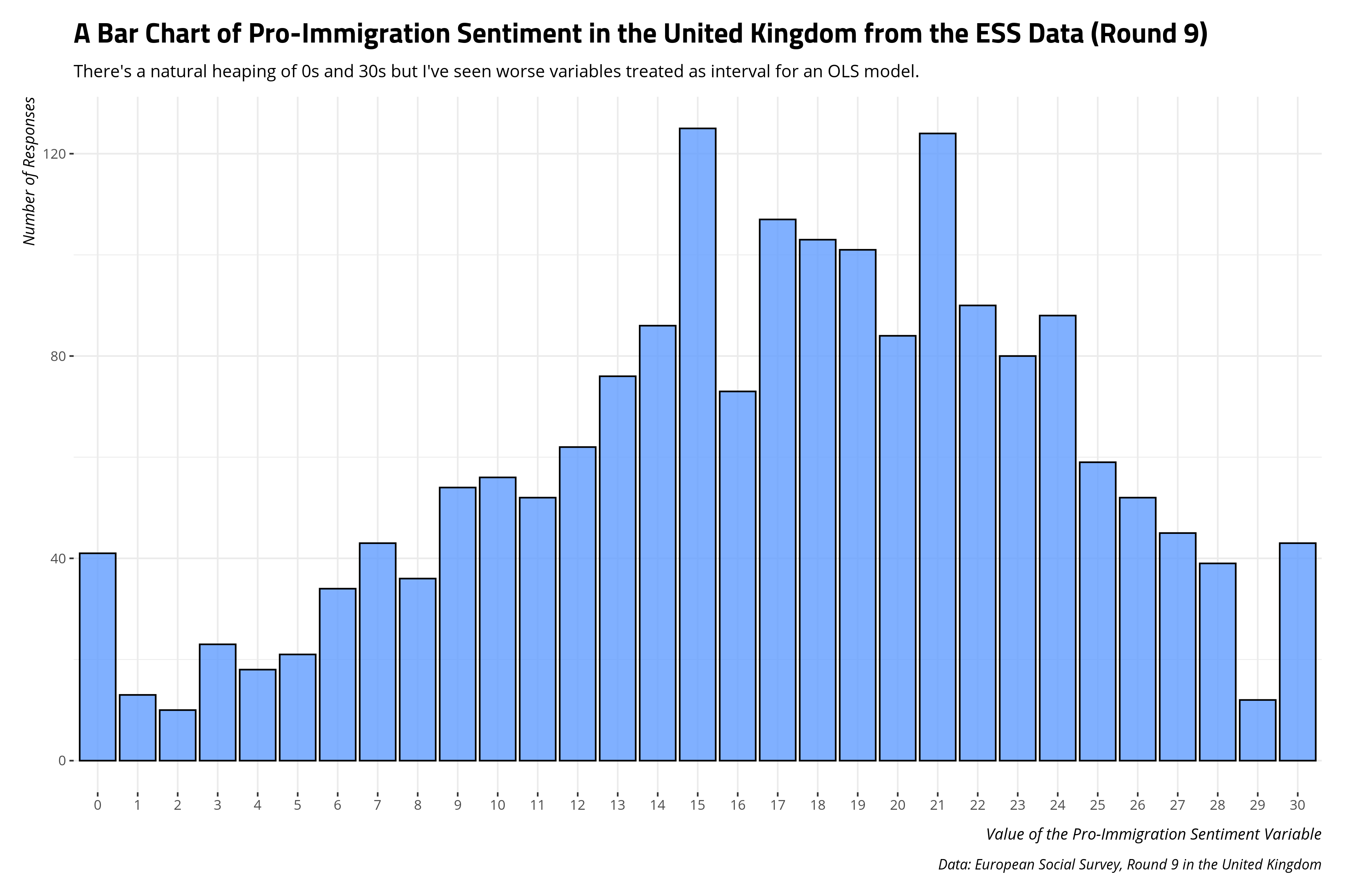
A simple bar chart should suffice to see what weirdness may emerge from the measure. Potential skew is more easily discerned graphically. In this case, there is a small natural heaping of 0s and 30s at the tail end of the distribution, but I’ve seen worse/weirder-looking variables treated as interval for the sake of calculating means or running a simple linear model. I would feel comfortable treating this variable as interval and communicating means from it.
ESS9GB %>%
  group_by(immigsent) %>% # group_by unique values of immigsent
  summarize(n = n()) %>% # return number of times that particular value was coded for variable
  na.omit %>% # drop NAs, which won't matter much here.
  ggplot(.,aes(as.factor(immigsent), n)) +  # create foundation ggplot
  # bar chart, with some prettiness
  geom_bar(stat="identity", alpha=0.8, color="black", fill="#619cff") +
  theme_steve_web() + # custom theme stuff
  labs(y = "Number of Responses",
       x = "Value of the Pro-Immigration Sentiment Variable",
       caption = "Data: European Social Survey, Round 9 in the United Kingdom",
       title = "A Bar Chart of Pro-Immigration Sentiment in the United Kingdom from the ESS Data (Round 9)",
       subtitle = "There's a natural heaping of 0s and 30s but I've seen worse variables treated as interval for an OLS model.")
What Can We Say About Pro-Immigration Sentiment in the UK from This Measure?
Let’s focus on the mean of the measure for the moment, which we calculated as 16.891 on that 31-point scale. Academics and journalists interpreting public opinion polls like this would summarize the sample mean we collected of the near 2,000 UK-born British respondents as our best estimate of the population mean of the entire country, knowing well that the responses in the survey sample are well below the actual population of the country (~66 million people). Here is an admittedly brief, incomplete, but workable rationale for why we say this. Interested students can read this recent blog post of mine, which talks about the normal distribution, central limit theorem, and sample inference in more detail.
First, central limit theorem says that infinity random samples of any size of a population of any size (say 66 million people) will produce sample means that follow a normal distribution. This holds even if you are doing infinity samples of 10 respondents from the target population. This would be a small sample size by itself, but, when done infinity times, this will still conform to the maxims of central limit theorem. The mean of sample means will be the actual population mean and random sampling error would equal the standard error of the sample mean. My recent blog post on central limit theorem offers a simulation that shows this.
Second, a random sample (like a survey I am using here) obtained from a target population (e.g. the population of the United Kingdom) provides the best means to guess attributes about the target population while knowing and appreciating two fundamental limitations. First, infinity random samples of a target population is obviously unrealistic. Second, gathering the entire population of the United Kingdom is also unrealistic in this context. So, a random sample of the population that has enough responses—typically around 1,000 responses—is a nice balance between tractable to obtain and sufficiently powered to reduce random sampling error.
Related, random sampling error is the chance differences between attributes of the sample and attributes of the target population. Simply, a truly random sample of the population is one in which respondents have an equal probability of being included or excluded from the sample. By chance, the composition of the sample will differ from the composition of the population (e.g. there might be more men relative to women in the sample than the true gender ratio of the United Kingdom). That random variation is unavoidable but does not, in theory, bias the information from the sample.
Finally, a normal distribution is a symmetrical, continuous function that resembles a familiar “bell curve.” Its peak is the arithmetic mean and its width is equal to the variance of the data. More interestingly, the probability of any one particular value is effectively zero (since it’s a continuous function) but the area underneath the familiar “bell curve” of the normal distribution constitutes the full domain of possible responses. That sums to 1 (i.e. the full domain of probabilistic outcomes). The symmetrical component is important too since -x is as far from the center of the distribution as x. With that in mind, researchers have found that 68% of the responses are within one standard unit on either side of the mean of the distribution. 95% are within 1.96 (“about 2”) standard units on either side of the mean. This allows us, importantly, to make inferential claims.
Inference By “Ruling Things Out”
These concepts will allow us to make inferential claims about pro-immigration sentiment in the United Kingdom. However, our inferential claims are limited and modest. Namely, we say our sample mean from the United Kingdom is our “best estimate” about the population mean of the entire country. Further, the inferences we make are less about saying what the “true” population mean is and it’s more about “ruling out” other alternatives as highly unlikely, given what we know from central limit theorem and the properties of a normal distribution.
Let’s illustrate this by reference to one of my favorite teachable moments for students; assessing a claim born from a hasty generalization. Let’s also set up some context by looking at the regional means across the entire United Kingdom on this data. One cool thing about the ESS data is respondents are also coded by the particular region of the UK in which they live. Again, I’ll condense the code that formats the table but this code will produce the results you see in the R console.
ESS9GB %>%
  mutate(region = as_factor(region)) %>% # extract more meaningful regional label from the data
  group_by(region) %>% # group by the region
  # get regional means
  summarize(meanimmigsent = round(mean(immigsent, na.rm=T), 3)) %>%
  # order from highest pro-immigration sentiment to lowest.
  arrange(-meanimmigsent)
| Region | Average Pro-Immigration Sentiment |
|---|---|
| Scotland | 18.503 |
| London | 17.982 |
| South East (England) | 17.858 |
| South West (England) | 17.564 |
| East of England | 17.399 |
| Northern Ireland | 17.333 |
| Yorkshire and the Humber | 16.634 |
| East Midlands (England) | 16.430 |
| Wales | 15.839 |
| West Midlands (England) | 15.562 |
| North West (England) | 15.513 |
| North East (England) | 14.650 |
The results here do not seem particularly surprising. Scotland and London emerge as having the highest pro-immigration sentiment. North East England, a region that at least has the reputation of being “Brexit central”, has the lowest pro-immigration sentiment. Their mean pro-immigration sentiment score is 14.650.
Let’s assume we encounter someone from North East who, given their local environment, is suspicious of our claim that the pro-immigration sentiment for the whole country is the 16.891 we report. S/he instead asserts that the true population sentiment is 14.650. In essence, this hypothetical person is making what we call a “hasty generalization”, in part inferring from a smaller sample size or their home environment rather than looking what is more typical of the entire population. How might you evaluate this claim, given your sample mean of 16.891?
The answer lay in some of the foundation stuff I briefly described above, especially in understanding the unique properties of a normal distribution and how well random samples of a large size approximate the population when infinity random samples are not possible. Thus, we can reframe this question as follows: how likely was our sample statistic of 16.891, given a proposed mean of 14.650?
First, you will need to calculate the standard error the sample mean, which is simply the standard deviation we just reported over the square root of the number of observations. You have that information in a table above. From that, you can calculate a 95% confidence interval. This is the interval through which 95% of all possible sample means would fall by chance, given what we know about the normal distribution. We can calculate this as follows, with a more polished result following the code:
ESS9GB %>%
  # Let's focus on what we want to get simpler calculations
  select(immigsent) %>% na.omit %>%
  # first, get the standard error
  summarize(mean = mean(immigsent),
            se = sd(immigsent, na.rm=T)/sqrt(n()),
            lb95 = round(mean - 1.96*se, 3),
            ub95 = round(mean + 1.96*se, 3))
| Sample Mean | Standard Error of the Sample Mean | 95% Conf. Int. (Lower Bound) | 95% Conf. Int. (Upper Bound) |
|---|---|---|---|
| 16.891 | 0.163 | 16.572 | 17.21 |
This information suggests we can have a fair bit of confidence around our sample estimate, given the standard deviation in the sample and the larger sample size. To be a bit more precise, while appreciating underlying sample probabilities, if we took 100 samples of this size (n = 1,850), 95 of those random samples would, on average, have sample means between about 16.572 and 17.210. That is nowhere near the 14.650 that is being proposed to us from this hypothetical person from North East. Already, the claim of 14.650 looks suspect given our random sample.
But, you can answer this question more directly by returning to the implications of the normal distribution. In other words, what is the probability of us observing our sample mean (16.891) if the true population mean were 14.650? You can answer this by calculating a z-score, which are how normal distributions on any scale typically get summarized.5 First compute the sample mean we got (16.891) minus the proposed mean (14.650), and divide it over the standard error of the sample mean (.163).
ESS9GB %>%
  # Let's focus on what we want to get simpler calculations
  select(immigsent) %>% na.omit %>%
  summarize(samplemean = mean(immigsent),
            se = sd(immigsent)/sqrt(n()),
            proposed = 14.650,
            zscore = (samplemean - proposed)/se)
| Sample Mean | Standard Error of the Sample Mean | Proposed Mean | z-score |
|---|---|---|---|
| 16.891 | 0.163 | 14.65 | 13.748 |
The z-score that emerges from this calculation is 13.748, meaning our sample statistic is more than 13 standard errors away from the proposed mean of 14.650. You can show how unlikely this is with a normal distribution. Consider the standard normal distribution below. This distribution has a mean of zero, for simplicity’s sake, and we observe that 68% of all values are with one standard unit from the mean of zero, 90% of all values are within about 1.645 standard units from the mean of zero, and 95% of all values are within about 1.96 standard units from zero. Further, 99% of the distribution is within about 2.58 standard units on either side of the distribution. The z-score we calculated of 13.748 won’t even appear on the plot.
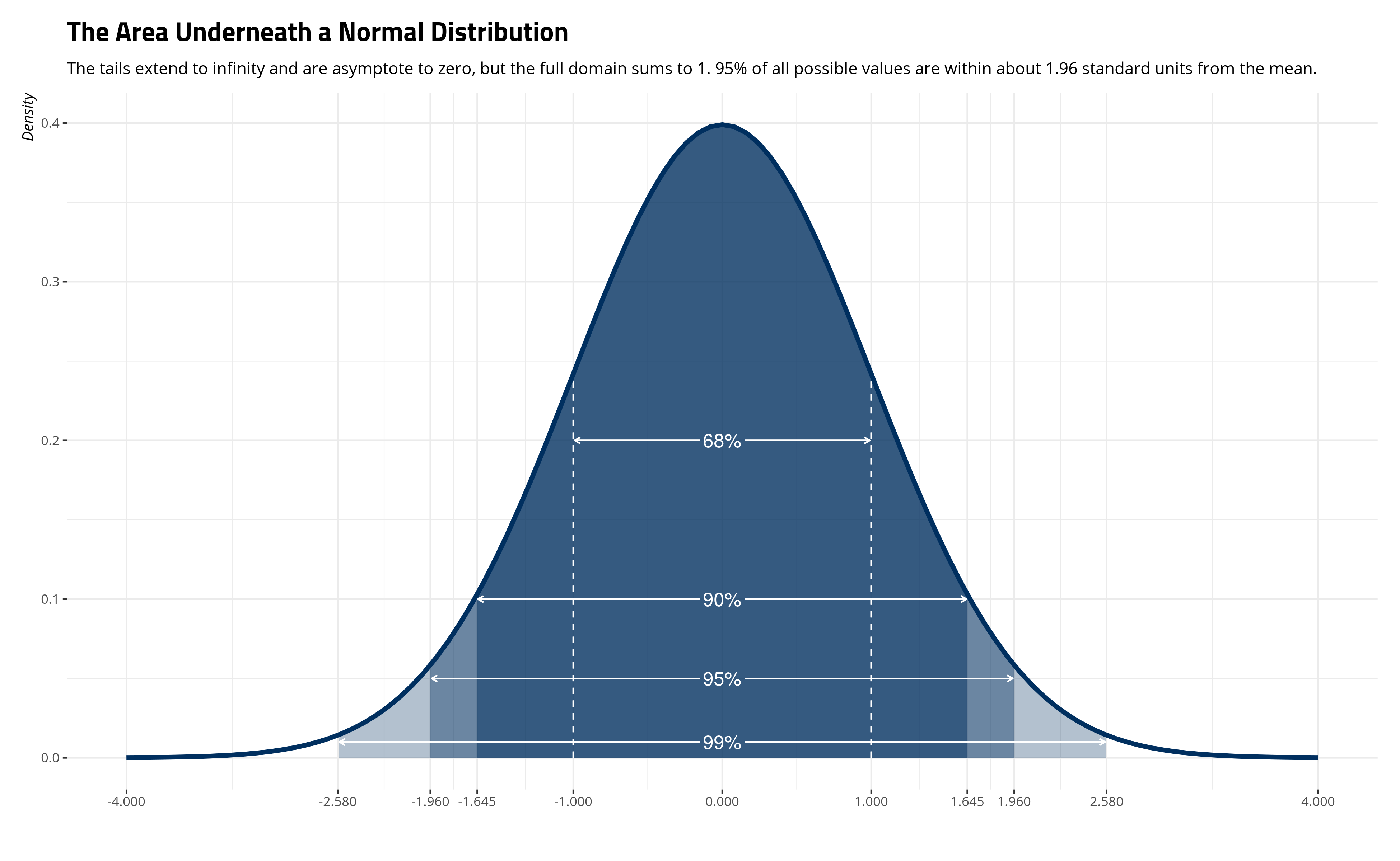
This graph will help us understand just how rare our z-score is. Consider that if 95% of the normal distribution is within about 1.96 standard units of the mean of the distribution, than 5% rests outside it. It is highly unlikely that we would find something outside 1.96 standard units on either side of the mean; indeed, we would only find something that extreme about 5% of the time, on average. Likewise, we can use a basic R calculation—2*pnorm(-abs(13.748))—to see what is the p-value associated with the z-score in a normal distribution.
2*pnorm(-abs(13.748)) # two-sided in this context
#> [1] 5.235696e-43
For context, that is going to be 42 zeroes after the decimal and before any other number. Formally, the probability of us observing our sample mean (16.891) with that z-score (13.748), given the true population mean is 14.650 is 5.2356956 × 10-43. Informally, that probability is effectively zero and converging on a near impossibility.
Here’s how we proceed with this information: we reject the claim that the true population mean is 14.650 and suggest our sample mean is closer to what the true population mean is. The likelihood of us observing it is almost zero if the true population mean were 14.650, but the result becomes much more probable if our sample mean is closer to what the true population mean is. Simulations I’ve done for my undergraduate quantitative methods class shows how this works even when you do know the population mean. To be clear, we are not saying the true population mean is actually our sample mean. The true population mean in this context is ultimately unknowable, but inference in this context comes not in saying what “is” but in ruling out things as highly unlikely to be true. In this case, we are suggesting this hypothetical person from North East is mistaken in an assertion that the North East mean is the population mean of the United Kingdom and that this hypothetical person is making a hasty generalization. Our sample mean (16.891) may not be strictly correct, but it’s much more likely to be closer to correct than the proposed population mean from the North East.
If you’re curious, our rule of thumb for making such a judgment call is the aforementioned 95% cutoff (i.e. z = 1.96). This is conservative enough but provides some more opportunity to do inference in an uncertain world than a more stringent threshold like 99%. However, even this decision for 95% is fundamentally arbitrary and it’s very much indebted to how Ronald Fisher pitched his test of significance. Toward that end, I highly recommend reading Stephen T. Ziliak and Deirdre N. McCloskey’s The Cult of Statistical Significance for both a history of this significance test as well as the pitfalls associated with it.6 However, this approach is still worthwhile for students to learn.
Regression as More Inference By “Ruling Things Out”
This same basic approach extends to regression. It would be impossible in the space and time allocated to fully explain all the properties of a linear regression, especially its assumptions and when those assumptions are violated. Those typically require whole textbooks—some classics even span almost 1,000(!) pages—and at least one semester of dedicated instruction. Instead, I will only note here as I did elsewhere on my blog almost six years ago that linear regression is a tool for understanding a phenomenon of interest (here: pro-immigration sentiment) as a linear function of some combination of predictor variables. The regression formula itself has a strong resemblance to the slope-intercept equation that students should remember from their secondary education. However, whereas students may have seen it before as y = mx + b, statisticians prefer a slightly different notation of the concept that is flexible and expands when there are more predictor variables included.
I’m going to keep this equation here very simple for two reasons. One, I want to minimize the extent of missing data that can emerge from including more variables. Two, the goal here is not to provide an exhaustive, all-encompassing explanation for pro-immigration sentiment in the United Kingdom. Instead, the goal here is to use it as a jumping-off point for students to learn how to read a regression table. So, we’re going to model pro-immigration sentiment as a function of some basic stuff (column names in the data noted in parentheses with typewriter text): the respondent’s age (in years) (agea), whether the respondent is a woman (gndr), how many years the respondent spent getting an education (eduyrs), whether the respondent is unemployed (but actively seeking work) (uempla), the respondent’s household net income as deciles (hinctnta), and the respondent’s ideology on an 11-point left-right scale (lrscale).7
First things first in looking at or running a regression: look at your data and recode as necessary. In this case, we should note the gndr variable is one where men are 1 and women are 2. We should recode that to be men = 0 and women = 1. In almost every survey application, gender is a binary (“dummy”) variable. These should always have a zero.
ESS9GB %>%
  # recode gndr, and make it a different variable (female)
  mutate(female = gndr - 1) -> ESS9GB
Next, we’re going to treat the immigsent variable as a linear function of these independent variables. Informally, immigsent = agea + female + eduyrs + uempla + hinctnta + lrscale + e. More formally:
I want to briefly note two things about this equation, stylized as it is. First, each of those predictors can clearly have different effects on immigsent, the dependent variable of immigration sentiment. That’s in part what we’re trying to tease out in a regression model and it’ll be something I highlight in the summary below. Second, the \(i\) notation you see is to denote the individual observation (i.e. individual survey respondent in our data). The values of a given variable for a particular respondent will vary but the estimated effects of a given variable on immigration sentiment (i.e. \(\beta\)) will be the same for all observations. Third, pay careful attention to that \(\epsilon\) term. We call that an “error term” or the “residuals” from the regression. Basically, \(\epsilon\) isn’t a predictor of interest. It represents everything that’s not included in our model that explains the variation in immigration sentiment that our linear function won’t capture. Without sidetracking too much into a discussion of minimizing the sum of squares (i.e. “ordinary least squares”) in regression, we expect the linear regression to draw a line of best fit through the data, but it won’t 100% capture every point in the data. The difference between what our regression predicts for a particular observation and the value of the particular observation is that “residual” or “error.”
Running a linear regression in R is simple. The commands below will do it while some code I hide will format the tables I present. Again, check the _rmd file.
M1 <- lm(immigsent ~ agea + female + eduyrs + uempla + hinctnta  + lrscale, data=ESS9GB)
summary(M1)
| Dependent variable: | |
| Pro-Immigration Sentiment | |
| Age | -0.002 |
| (0.010) | |
| Female | -0.248 |
| (0.338) | |
| Years of Education | 0.488*** |
| (0.049) | |
| Unemployed | -1.102 |
| (1.204) | |
| Household Income (Deciles) | 0.338*** |
| (0.061) | |
| Ideology (L to R) | -0.583*** |
| (0.088) | |
| Constant | 11.655*** |
| (1.061) | |
| Observations | 1,454 |
| Note: | *p<0.1; **p<0.05; ***p<0.01 |
| Data: ESS, Round 9 (United Kingdom) | |
Here I’m inclined to parrot what I noted in my guide from six years ago. The tl;dr (if you will) for students looking at a regression table is to take inventory of three things.
- The numbers inside parentheses next to a variable.
- The numbers not in parentheses next to a variable.
- Some of those numbers not in parentheses have some asterisks next to them.
Let’s break those down, starting with the second item.
The Regression Coefficient
The number you see not in parentheses is called a regression coefficient. The regression coefficient provides the expected change in the dependent variable (here: immigsent) for a one-unit increase in the independent variable.
I encourage students new to regression to observe two elements of the regression coefficient. Namely, is it positive or negative? A positive coefficient indicates a positive relationship. As the independent variable increases, the dependent variable increases. Also, the dependent variable decreases as the independent variable decreases.
A negative coefficient indicates a negative relationship. As the independent variable increases, the dependent variable decreases. A negative relationship also indicates that the dependent variable increases as the independent variable decreases.
In our case, we can see two intuitive stories emerge. Higher levels of education (i.e. more years of education) coincide with more pro-immigration sentiment. As years of education go up, so too does the pro-immigration sentiment variable. That’s a positive relationship. Ideological placement further to the right on an 11-point left-right scale coincides with lower levels of pro-immigration sentiment. Conversely, those who place themselves closer to the ideological left are more likely to have higher levels of pro-immigration sentiment. As one goes up, the other goes down, and vice-versa. That’s a negative relationship.
The Standard Error
The number in parentheses is called a standard error. For each independent variable, we expect to be wrong in our predictions. It’s intuitive that better educated people are more likely to have more positive sentiment toward immigrants/immigration and it’s intuitive that those who place themselves further to the ideological right will have lower levels of positive sentiment toward immigrants/immigration than those who place themselves further to the ideological left. However, predictions are almost never 100% and the line of best we can draw through the data won’t perfectly capture every single data point. The standard error is our estimate of the standard deviation of the coefficient.
However, the standard error is not a quantity of interest by itself. It depends on the relationship with the regression coefficient. This leads us to the third item of interest.
The Asterisks
The asterisks in a regression table correspond with a legend at the bottom of the table. In our case, one asterisk means “p < .1”. Two asterisks mean “p < .05”; and three asterisks mean “p < .01”. What do these mean?
Asterisks in a regression table indicate the level of the statistical significance of a regression coefficient. The logic here is built off the principle of random sampling we discussed above. If there truly is no difference between (for example) men and women in their pro-immigration sentiment, and if increasing years of education truly had no effect on pro-immigration sentiment, then how likely would we get the “draw” that suggested the effects we observed?
The answer here is “unlikely” for the years of education, household income, and ideology variables. Those are “statistically significant”, which means their true effects are highly unlikely to be zero effect in the population given the sample we collected and analyzed.
Think of what’s at stake here as equivalent to the exercise above, where we dismissed the likelihood of a “true” population mean being what we observed in North East based off the random sample we collected. We communicated that by getting a z-score that subtracted the proposed mean from our collected mean and divided that difference over the standard error of the sample mean. However, what’s happening here is a bit more simple than that. We’re testing our regression coefficient against a hypothetical claim of zero. Thus, we can get our standardized statistic by dividing the regression coefficient over the standard error. It’s that simple.
What emerges in the linear regression context is a t-statistic, which is a close cousin to the z-score.8 Briefly, z-scores are drawn from a normal distribution whereas t-statistics come from Student’s t-distribution. Student’s t-distribution closely resembles a normal distribution, but with fatter tails with fewer degrees of freedom. In the regression context, “degrees of freedom” is the number of observations (n: 1,454) minus the number of parameters the model is estimating (k, which is 7). This might seem like a lot of changes but more degrees of freedom collapses Student’s t-distribution to a normal distribution, and does so pretty quickly (all things considered).
More importantly, the process of inference is exactly the same. Divide the regression coefficient over the standard error. If the absolute value of that is about 1.96, you can reject the proposed claim of zero effect and substitute that your negative or positive relationship is closer to what the true effect in the population is.
tidy() from the {broom} package will do this for us, fortunately. Some extra code I hide will make it prettier to view. I’ll also omit the constant (or y-intercept) from this because the constant or y-intercept is just the estimate of y when all predictors are set to zero.
tidyM1 <- tidy(M1) # from the {broom} package
tidyM1
| Variable | Coefficient | Standard Error | t-Statistic | p Value |
|---|---|---|---|---|
| Age | -0.002 | 0.010 | -0.183 | 0.855 |
| Female | -0.248 | 0.338 | -0.735 | 0.462 |
| Years of Education | 0.488 | 0.049 | 10.007 | 0.000 |
| Unemployed | -1.102 | 1.204 | -0.915 | 0.360 |
| Household Income (Deciles) | 0.338 | 0.061 | 5.498 | 0.000 |
| Ideology (L to R) | -0.583 | 0.088 | -6.611 | 0.000 |
The statistical significance of years of education, household income, and ideology are easily discernible. The likelihood of observing those effects if the true effect in the population were zero is itself zero. So, we reject those claims of zero relationship and suggest education and household income have positive effects on pro-immigration sentiment while increasing ideology to the political right has a negative effect on pro-immigration sentiment.
Here, though, it might make sense to belabor why we should say age, gender, and unemployment have no effect, or have “statistically insignificant” effects, on the immigration sentiment variable. Let’s look at age first. To be clear, we observe a negative effect that prima facie implies that older Brits have lower levels of pro-immigration sentiment than younger Brits (i.e. a negative relationship). However, the probability of us observing this negative effect, if there was truly no effect of increasing age or differences in pro-immigration sentiment by age, is .855. That is obviously very probable. So, we cannot dismiss a counterclaim of zero relationship because the coefficient and standard error we collected are quite probable (.855) if the true effect were zero.
This type of statement might be more accessible in the context of unemployment and gender, which are binary indicators that look for differences between the not-unemployed/unemployed and men/women (respectively).9 In our sample, women were, on average, likely to exhibit lower levels of pro-immigration sentiment compared to men. However, the probability of observing this difference if there were truly no differences between men and women is .462. That’s definitely a probable result, so we cannot dismiss a claim of zero relationship. The same holds for the unemployed. The negative effect for the unemployed variable makes sense in the political economy of immigration framework; the unemployed seem to have lower levels of pro-immigration sentiment. However, the probability of us observing that effect if the true effect is zero is .360. That’s a probabilistic result, so we cannot dismiss a counterclaim that there is no effect of being unemployed relative to not being unemployed on pro-immigration sentiment.
However, notice the process of inference is the same as above. What emerges from our regression is an estimate, and our “best guess”, of the effect these predictors have on pro-immigration sentiment as we measured it. An effect that is “statistically significant” is one that we are confident is not zero effect. Much like above, inference comes not necessarily in saying what something “is.” Inference as we practice it is ruling out counterclaims as highly unlikely, given the sample we collected and analyzed.
I’ll close this section by noting, as I did in my guide from 2014, that a student reading a regression table can probably just focus on the “stars.” This bit of extra work extracting t-statistics and the associated p-values will better emphasize why something that is “statistically significant” can permit us to confidently reject a claim of zero relationship and why an effect that is “statistically insignificant” is in fact a “probable draw” given a counterclaim of zero relationship. However, “stargazing” (i.e. looking for asterisks) is acceptable because they’ll communicate that information in as many words.
Some Concluding Thoughts
I want to offer the following concluding thoughts, some of which will echo my thoughts on my guide from 2014.
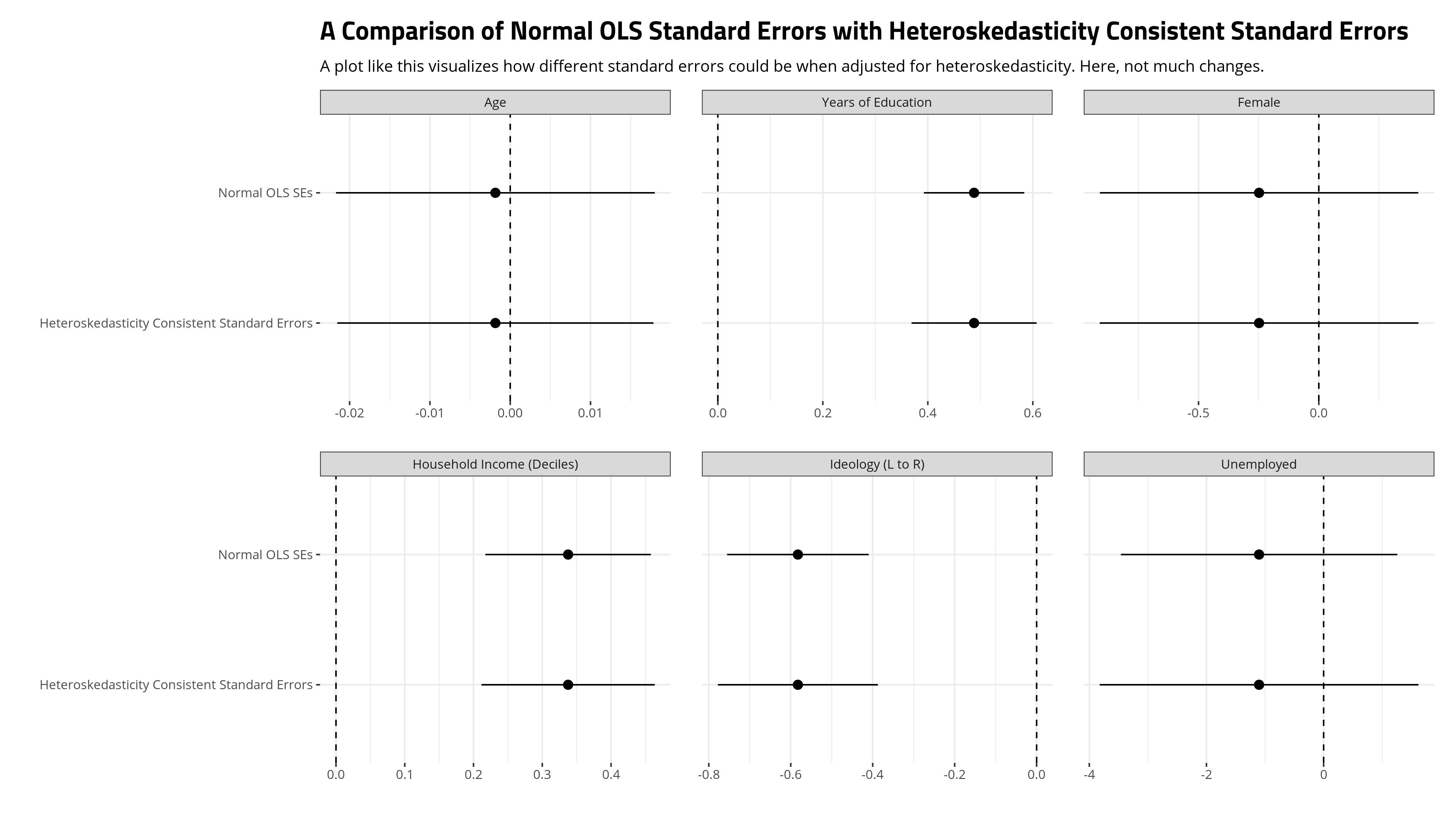
First, be mindful of the distribution of the dependent variable. In this application, we’re treating this 31-point composite index as interval and I think it’s reasonable to do so. The distribution of the measure didn’t look too wonky, all things considered. However, variables with a huge skew problem or just a handful of responses (e.g. five-item Likerts, binary responses) will either break some of the underlying assumptions of a linear regression or will produce nonsensical quantities of interest. Basically, look at your data and look at your model. In this case, maybe there’s a heteroskedasticity concern, but a heteroskedasticity correction I run (quietly) and report here suggest no major concern for our coefficients. I have a lab script for my grad-level methods class that shows how flexible you can get with heteroskedasticity corrections. You could also bootstrap your standard errors, which I show how to do here in detail. I’m electing for a simpler heteroskedasticity correction. You can see in the source file what exactly I did here (via the {sandwich} package).
Second, be mindful of the independent variables. Put another way: statistically significant is not itself “significant”. It’s easy to conflate “significant” with “large” or “very important.” However, the test of statistical significance is misleading because it’s really a test of prescision and discernibility from zero. I’ll always bring up that “statistically signficant” made a prestigious list of terms that scientists wish the general public would stop misusing.
“Statistically significant” is one of those phrases scientists would love to have a chance to take back and rename. “Significant” suggests importance; but the test of statistical significance, developed by the British statistician R.A. Fisher, doesn’t measure the importance or size of an effect; only whether we are able to distinguish it, using our keenest statistical tools, from zero. “Statistically noticeable” or “Statistically discernible” would be much better.
Thus, be very careful in assuming that coefficient size is necessarily an indicator of the “strength” of an effect. None of those variables share a common scale, beyond the binary indicators, so a comparison of coefficients would be misleading. However, one way around this is through Gelman’s (2008) recommendation to scale every non-binary predictor by two standard deviations rather than just one standard deviation. Dividing by two standard deviations allows continuous predictors to be roughly similar in scale to binary variables. The benefits to this are multiple. The shape of the distribution of the predictors is unchanged, and the associated t-statistics will be unchanged as well. But, the coefficients now communicate magnitude changes across approximately 47.7% of the data in a particular predictor variable. Sometimes it’s more important to know magnitude changes (e.g. the effect of going from 54 to 88 in age) rather than incremental changes (e.g. the effect of going from 18 to 19 in age).
Everything is centered on zero as well so the “constant” (or y-intercept) now communicates the expected value of y for a typical case approximating the mean. The first model, which is not standardized, gives us an estimate of y to be about 11.655 for a person who is a 1) zero-years-old(!) 2) male who 3) was never educated(!) and self-identifies as 4) furthest to the ideological left, but is 5) currently employed even if 6) their household income is zero(!) on a 1:10 scale. That estimate for a y-intercept is useless, as the exclamation points I add suggest. When standardized, the y-intercept of 17.269 gives us the estimated value for an employed man of average age, education, income, and ideology. That y-intercept is much more useful the extent to which it conveys a quantity of interest for an observation that is much more likely to actually exist.
More to the point, binary and non-binary inputs are now roughly on the same scale, allowing for a preliminary comparison of coefficients. The r2sd() function in my {stevemisc} package will do this standardization.
ESS9GB %>%
  mutate(z_agea = r2sd(agea),
         z_eduyrs = r2sd(eduyrs),
         z_hinctnta = r2sd(hinctnta),
         z_lrscale = r2sd(lrscale)) -> ESS9GB

M2 <- lm(immigsent ~ z_agea + female + z_eduyrs + uempla + z_hinctnta  + z_lrscale, data=ESS9GB)
The results from the regression does offer some preliminary evidence that the years of education variable has the strongest magnitude effect. It is also the most precise. On a common scale, the absolute value of the effects of ideology and household income look comparable as well whereas that may not have been obvious in the unstandardized model.
| Pro-Immigration Sentiment | ||
| Unstandardized Coefficents | Standardized Coefficients | |
| (1) | (2) | |
| Age | -0.002 | -0.068 |
| (0.010) | (0.372) | |
| Female | -0.248 | -0.248 |
| (0.338) | (0.338) | |
| Years of Education | 0.488*** | 3.544*** |
| (0.049) | (0.354) | |
| Unemployed | -1.102 | -1.102 |
| (1.204) | (1.204) | |
| Household Income (Deciles) | 0.338*** | 2.007*** |
| (0.061) | (0.365) | |
| Ideology (L to R) | -0.583*** | -2.267*** |
| (0.088) | (0.343) | |
| Constant | 11.655*** | 17.269*** |
| (1.061) | (0.243) | |
| Observations | 1,454 | 1,454 |
| Note: | *p<0.1; **p<0.05; ***p<0.01 | |
| Data: ESS, Round 9 (United Kingdom). | ||
Further, as another word of caution, more asterisks do not mean more “significance.” Greater levels of statistical significance (i.e. more “stars”) suggest only more precise estimates, not bigger or “more important” effects. Significance is an assessment only of precision and discernibility from some other counterclaim (of zero in the regression context).
Finally, I offer this humbly, only as a companion to a presentation to some politics students in the United Kingdom. I do not intend it to be exhaustive of all the covariates of immigration attitudes; it clearly is not. I offer it only as a complement to students on how to approach social/political science topics quantitatively and how to evaluate quantitative evidence presented to them. There’s so much more a researcher could do with these data, whether it’s exhausting all sources of omitted variable bias potentially present or more fully explicating some of the regional variation in a mixed effects modeling approach. Explore the data with that in mind. Interested students from that presentation I was slated to give are free to reach out to me as well with additional inquiries on these data.
-
I’ve since published
{stevedata}on CRAN, which has theESS9GBdata I’m creating here. ↩ -
I tend to favor the SPSS binaries over the Stata binaries as an R user because the SPSS binaries are less likely encounter character encoding issues than the Stata binaries (from my experience) when calling the data into R. This matters a lot for data outside the American context (again, from my experience). ↩
-
My scholarship in the American context strongly implies attitudes toward immigration are functions of attitudes on race. More sophisticated/rigorous analyses in the British context may want to incorporate that, but this more sophisticated/rigorous design falls outside the scope of the intended goal of this post/analysis. The primary goal here is to introduce students to a quantitative approach to understanding a social scientific topic, not necessarily to exhaust all the important covariates on immigration attitudes. ↩
-
A factor analysis I quietly ran returns factor loadings for each of .862 (the economy prompt), .919 (the culture prompt), and .953 (the better or worse place to live prompt) with a proportional variance of .832. ↩
-
In this application, a t-statistic would make more sense because we don’t know the population standard deviation. However, as I’ll belabor more below, a Student’s t-distribution is a close cousin to the normal distribution and, in this application, a simple one-parameter t-statistic with as many observations we have will be basically the z-score since Student’s t-distribution collapses to a normal distribution pretty quickly with more degrees of freedom (i.e. we have 1,850 observations and just one parameter we’re trying to estimate). Observe the z-score (5.2356956 × 10-43) and the t-statistic (5.640342 × 10-41) for this simple exercise. However, we all learn about z-scores before we learn about the t-statistic, so I think getting the z-score by treating the sample standard deviation as the population standard deviation is fair game here. After all, William Sealy Gosset—aka “Student”—developed his pseudonymous Student’s t-distribution for making inferential claims from sample sizes as few as 3. ↩
-
Related to this conversation, but the 68-90-95-99 rule is technically wrong as well. For example, 68% of the distribution is within about 0.9944579 standard units from zero in a normal distribution, 90% of the distribution is within about 1.6448536 standard units from zero, 95% of the distribution is within about 1.959964 standard units while 99% of the distribution is within about 2.5758293 standard units from zero in the normal distribution. That much is immaterial here for this exercise the extent to which those cutoffs clearly approximate what they’re supposed to approximate. Still, some humility from academics would be warranted in evaluating p-values. ↩
-
Only about 1.9% of the sample self-identified as unemployed but actively seeking work. After some missing data in the other covariates, there are only 30 unemployed people in the sample. It’s worth noting this because there’s going to be considerable uncertainty around that estimate for that reason alone. ↩
-
Briefly, linear regression uses t-tests rather than z-scores because OLS responses have both a mean and a variance that must be estimated. The mean is normally distributed but the variance is independent of it. The fatter tails of Student’s t-distribution does well to capture this. Looking ahead to something like logistic regression (i.e. when the dependent variable is just 0 or 1), there is really just one parameter to estimate. Basically, the mean of a binary variable is the proportion of 1s (i.e. p) and the variance is p(1 - p). Thus, the variance is no longer independent of the mean and the normal distribution will suffice in place of Student’s t-distribution. ↩
-
“Not unemployed” is clunky language here but it’s technically accurate. “Unemployed” refers to those without a job but unable to find one despite actively looking. This would exclude, by definition, several other groups of people who are “unemployed” but not looking for work (e.g. students, stay-at-home parents). ↩
Disqus is great for comments/feedback but I had no idea it came with these gaudy ads.