Clever Uses of Relational (SQL) Databases to Store Your Wider Data (with Some Assistance from {dplyr} and {purrr})

- Postgres is a pretty powerful relational database system.
Last updated: 19 June 2021. The function described here is now db_lselect() in {stevemisc}. You can download this package on CRAN.
For some time, I’ve wrestled with how to elegantly store two data sets I use a great deal in my own research or navel-gazing. The first is the General Social Survey (GSS) and the second is the World Values Survey (WVS). The GSS contains 32 survey waves, done roughly every two years, spanning 1972 and 2018 in the United States. The temporal reach of the data are broadly useful for tracking trends in public opinion over time, but different questions come and go at different points in time. The data as I have it are not particularly long (64,814 rows), but they are very wide (6,108 columns). The data are well-annotated with variable labels too, which compounds how tedious it is to load and explore. The WVS (v. 1-6) is similarly gnarly to load. The data contains surveys of roughly 100 countries in 28 different years spanning 1981 to 2009. The data are mercifully more standardized across countries and waves than the GSS, but, at 348,532 rows and 1,445 columns, they too are tedious to load and explore. To this point, my experiences have suggested to say nuts to the native formats of these data and save them as R serialized data frames or serialize them with the {qs} package.
However, I’ve been wanting to dedicate more time to unpacking relational databases and using them more in my own workflow. My expertise with relational databases is mostly intermediate; I think I’m great with the rudimentary SELECT * FROM data WHERE foo HAVING bar LIMIT 0,10;. But, workflow around database systems feature more prominently in the private sector. Thus, a bit more SQL know-how is useful not only for students, but for me, just in case. Integrating SQL into my workflow around these two data sets in particular has been gnawing at me for a while. Here’s how I ended up doing it for both, preceded by a table of contents.
- Set Up PostgreSQL on Your Computer
- “Selectively Select” and Populate the Databases
- Harness
{dplyr}and{purrr}to Make the Most of These Databases
Set Up PostgreSQL on Your Computer
First, I installed PostgreSQL on my Ubuntu desktop. The most current stable release is already at version 13, though the default version in my Ubuntu 18.04.2 release is version 10. That much won’t matter for the task at hand. You could also use really any relational database (including MySQL), but PostgreSQL is just a bit more powerful than MySQL.
sudo apt-get update
sudo apt-get install postgresql-client-10 postgresql-common
Thereafter, I logged into the PostgreSQL server with the following sudo command in the terminal. Technically, you’re executing the psql program as if you were the default superuser postgres. You can (and perhaps should) create your own account with appropriate privileges, but this may require adjusting authentication methods.
sudo -u postgres psql
Next, I created two relational database shells to store these data.
CREATE DATABASE wvs;
CREATE DATABASE gss;
There’s a convoluted way of doing this entirely within PostgreSQL, but I’ll opt for R wrappers around these.
Load the GSS and WVS Data
Next, fire up an R session, load the GSS and WVS data, along with various packages to assist in the process. Do note that the versions of the data I have are from the {qs} package. I discuss these here. I also hate all-caps column names, so I made sure to put those in lowercase in the GSS data (but evidently forgot to do that for the WVS data). I’ll also note that some of the things I propose downstream are augmented by having a unique identifier for each observation in the data. I manually create that (uid) here.
library(tidyverse)
library(stevemisc)

WVS <- qs::qread("~/Dropbox/data/wvs/wvs6wave-20180912.qs") %>%
  rename_all(tolower) %>% mutate(uid = seq(1:n())) %>%
  select(s001, s002, uid, everything())
GSS <- qs::qread("~/Dropbox/data/gss/GSS_spss-2018/gss7218.qs") %>%
  mutate(uid = seq(1:n())) %>%
  select(year, uid, everything())
The process I propose leans on the group_split() function in {dplyr}. I’m going to split the data into multiple data frames by survey wave (in the WVS data) and survey year (in the GSS data). {dplyr} will return these as lists. Recall, however, the basic problem of the data. The problem of loading the data is in large part a function of how wide the data are. The width of the data comes from the temporal reach of each (and, in the case of the WVS, the spatial reach as well). Some questions appear at some points of time, but not others. The GSS, for example, asked questions about the 1972 election between Richard Nixon and George McGovern every year from 1973 to 1977. After 1977, the question no longer became interesting to ask. If, however, you load the data because you’re interested in more current topics, you’ll get that data too. So, for both the GSS and the WVS, I omit columns if all the responses were NA for the particular split. This requires defining a custom function, though.
“Selectively Select” and Populate the Databases
not_all_na <- function(x) any(!is.na(x))
Thereafter, I split the GSS and WVS data by these waves/survey years and select only the columns that are not completely missing/unavailable in a given wave/year. This is where some knowledge of {purrr} will emphasize how amazing the package is for tasks like these. The map() function is basically applying one function to six (in the WVS data) or 32 (in the GSS data) different data frames contained in the list.
WVS %>% haven::zap_labels() %>%
  group_split(s002) %>%
  map(~select_if(., not_all_na)) -> splitWVS


GSS %>%
  haven::zap_labels() %>%
  group_split(year) -> splitGSS

 # strip vector information out
splitGSS <- as.list(splitGSS)

splitGSS %>%
  # this will take a while...
  map(~select_if(., not_all_na)) -> splitGSS
Observe what this does to the data in the case of the World Values Survey. Do note the dimensions I report here omit the unique identifier (uid) I created.
| Data | Number of Rows | Number of Columns |
|---|---|---|
| WVS (Waves 1-6) | 348,532 | 1,445 |
| WVS (Wave 1) | 13,586 | 187 |
| WVS (Wave 2) | 24,558 | 480 |
| WVS (Wave 3) | 77,818 | 339 |
| WVS (Wave 4) | 59,030 | 434 |
| WVS (Wave 5) | 83,975 | 417 |
| WVS (Wave 6) | 89,565 | 398 |
Thereafter, I’m going to use R as a wrapper to connect to PostgreSQL, starting with the WVS data.
wvspgcon <- DBI::dbConnect(RPostgres::Postgres(), dbname="wvs")
Here’s what I’m going to do next. My splitWVS object is split by the survey waves (s002), which are minimally 1, 2, 3, 4, 5, and 6. In this wvs PostgreSQL database, those will be my table names coinciding with the individual survey waves I split. The next part just loops through the data and creates those tables with those names.
wvs_waves <- seq(1:6)

for (i in 1:length(splitWVS)) {
  l <- as.character(wvs_waves[i])
  copy_to(wvspgcon, as.data.frame(splitWVS[[i]]), l,
          temporary=FALSE)

}
From there, the real benefits of relational databases and {dplyr}’s interface with them shine. The data load quickly and the user can explore the data as “lazily” as possible. Observe by just spitting out the entire sixth survey wave as a tibble:
tbl(wvspgcon, "6")
#> # Source:   table<6> [?? x 399]
#> # Database: postgres [steve@/var/run/postgresql:5432/wvs]
#>     s001  s002    uid  s003 s003a  s006    s007  s007_01 s009  s009a  s012  s013
#>    <dbl> <dbl>  <int> <dbl> <dbl> <dbl>   <dbl>    <dbl> <chr> <chr> <dbl> <dbl>
#>  1     2     6 258968    12    12     1  1.21e8   1.21e8 "   … -4       NA     2
#>  2     2     6 258969    12    12     2  1.21e8   1.21e8 "   … -4       NA     1
#>  3     2     6 258970    12    12     3  1.21e8   1.21e8 "   … -4       NA     1
#>  4     2     6 258971    12    12     4  1.21e8   1.21e8 "   … -4       NA     2
#>  5     2     6 258972    12    12     5  1.21e8   1.21e8 "   … -4       NA     1
#>  6     2     6 258973    12    12     6  1.21e8   1.21e8 "   … -4       NA     3
#>  7     2     6 258974    12    12     7  1.21e8   1.21e8 "   … -4       NA     2
#>  8     2     6 258975    12    12     8  1.21e8   1.21e8 "   … -4       NA     2
#>  9     2     6 258976    12    12     9  1.21e8   1.21e8 "   … -4       NA     2
#> 10     2     6 258977    12    12    10  1.21e8   1.21e8 "   … -4       NA     1
#> # … with more rows, and 387 more variables: s013b <dbl>, s016 <dbl>,
#> #   s017 <dbl>, s017a <dbl>, s018 <dbl>, s018a <dbl>, s019 <dbl>, s019a <dbl>,
#> #   s020 <dbl>, s021 <dbl>, s021a <dbl>, s024 <dbl>, s024a <dbl>, s025 <dbl>,
#> #   s025a <dbl>, a001 <dbl>, a002 <dbl>, a003 <dbl>, a004 <dbl>, a005 <dbl>,
#> #   a006 <dbl>, a008 <dbl>, a009 <dbl>, a029 <dbl>, a030 <dbl>, a032 <dbl>,
#> #   a034 <dbl>, a035 <dbl>, a038 <dbl>, a039 <dbl>, a040 <dbl>, a041 <dbl>,
#> #   a042 <dbl>, a043_f <dbl>, a043b <dbl>, a098 <dbl>, a099 <dbl>, …
{dplyr}’s interface with relational databases like PostgreSQL is not exhaustive, but it is pretty comprehensive. For example, I could see how many countries are in the first and sixth survey wave.
tbl(wvspgcon, "1") %>%
  # s003 = country code
  select(s003) %>%
  distinct(s003) %>% pull() %>% length()
#> [1] 10

tbl(wvspgcon, "6") %>%
  select(s003) %>%
  distinct(s003) %>% pull() %>% length()
#> [1] 60
Now, it’s time to do the same with the GSS data. Here, though, the tables in the database are named by the survey year.
gsspgcon <- DBI::dbConnect(RPostgres::Postgres(), dbname="gss")

GSS %>% distinct(year) %>% pull(year) %>% as.vector() -> gss_years

for (i in 1:length(splitGSS)) {
  l <- as.character(gss_years[i])
  copy_to(gsspgcon, as.data.frame(splitGSS[[i]]), l,
          temporary=FALSE)

}
Harness {dplyr} and {purrr} to Make the Most of These Databases
The next step is to harness {dplyr} and especially {purrr} to make the most of storing the data in databases like this. The only real downside to what I propose here is you’re going to have to get somewhat comfortable with these data in order to more effectively maneuver your way around them in this format. That’ll come with time and experience using the data in question.
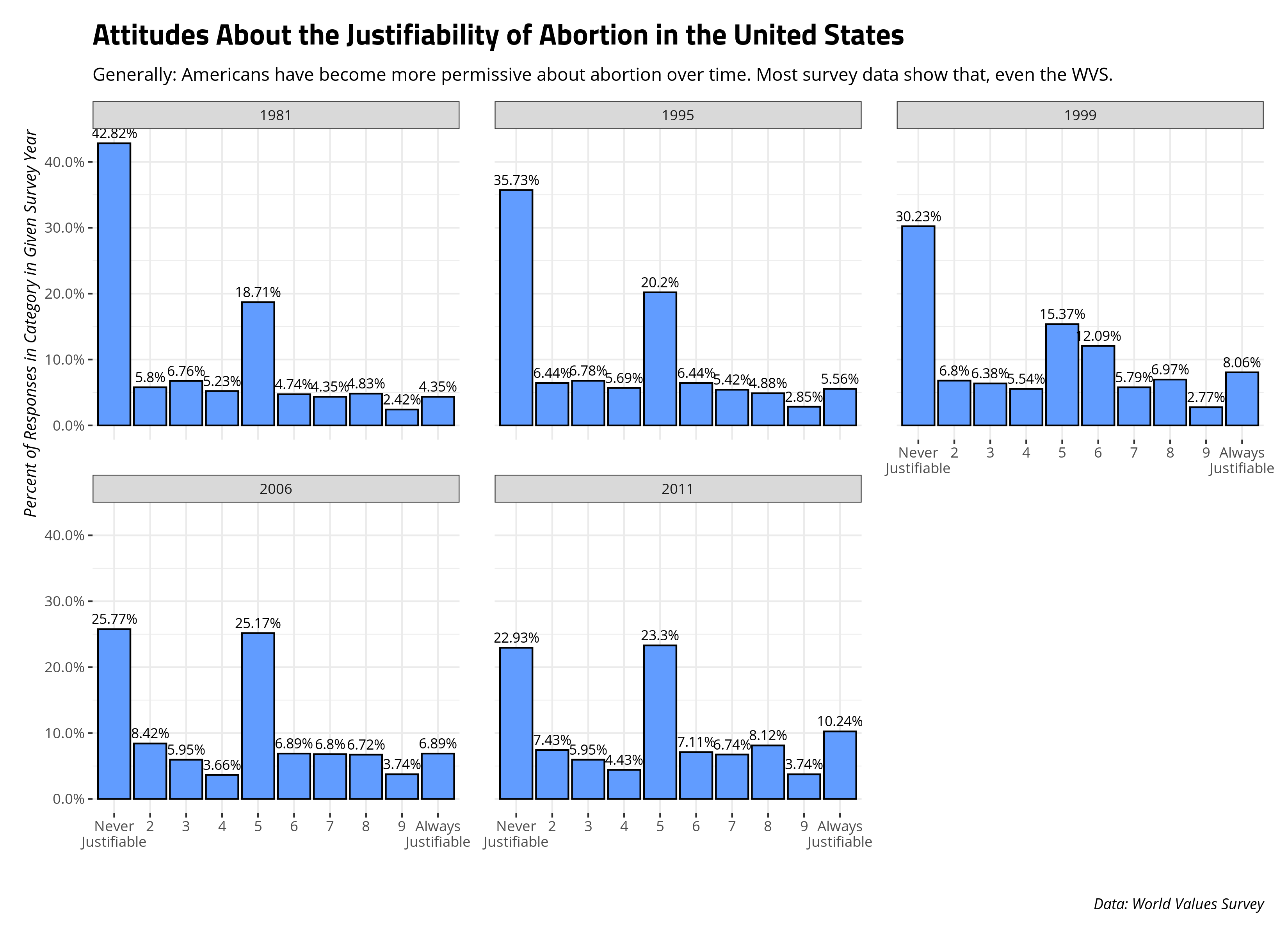
Here’s one example. I routinely use the WVS data to teach methods students about various methodological topics with an application to various political issues. One hobby horse of mine is teaching students about abortion opinions in the United States. From experience, I know the United States’ country code (s003) is 840 and that the WVS asks about the justifiability of abortion on a 1-10 scale where 1 = never justifiable and 10 = justifiable. That particular prompt appears as f120 in the data. Let’s assume I wanted to grab just those data from all six survey waves from the database.1 How might I do that? Here, a native {purrr} solution is not so straightforward since lists of data frames are alien concepts in the SQL world.
However, a database of tables is a close corollary, and that is native in SQL. So, here’s a clever workaround in {purrr}. First, create a vector of characters coinciding with the names of the tables in the database. This isn’t too hard in the WVS database I created since the names coincide with the survey waves.
waves <- as.character(seq(1:6))
Now, let’s write a function in map() that will do the following. For each of the waves specified in the waves character, we’re going to filter the observations to just the United States (s003 == 840) and select (for clarity) just the survey wave (s002), the country code (s003 == 840), the survey year (s020). More importantly, we’re going to grab the respondent’s attitude about the justifiability of abortion on a 1-10 scale (f120) and the unique identifier (uid). Then, we’re going to condense them into a single “lazy” tibble (f120_query) using the union() function. Here, I want to note, is where having the unique identifier for each row is useful. If you don’t have the unique identifier, the ensuing query will produce a row of 55 observations for each unique combination of survey wave, country code, survey year, and abortion opinion across all waves. We want the raw data, not a summary of the unique combination of values in them.
waves %>%
  map(~{
    tbl(wvspgcon, .x) %>%
      filter(s003 == 840) %>%
      select(uid, s002, s003, s020, f120)
  }) %>%
  reduce(function(x, y) union(x, y)) -> f120_query

f120_query
#> # Source:   lazy query [?? x 5]
#> # Database: postgres [steve@/var/run/postgresql:5432/wvs]
#>       uid  s002  s003  s020  f120
#>     <int> <dbl> <dbl> <dbl> <dbl>
#>  1 339053     6   840  2011     1
#>  2 337342     6   840  2011     6
#>  3 112198     3   840  1995     3
#>  4 112244     3   840  1995     9
#>  5 171210     4   840  1999     3
#>  6 113216     3   840  1995     3
#>  7 337527     6   840  2011     7
#>  8  13513     1   840  1981     8
#>  9 253940     5   840  2006     1
#> 10 337960     6   840  2011     8
#> # … with more rows
If you’d like, you can see underlying SQL query here.
show_query(f120_query)
#> <SQL>
#> (((((SELECT "uid", "s002", "s003", "s020", "f120"
#> FROM "1"
#> WHERE ("s003" = 840.0))
#> UNION
#> (SELECT "uid", "s002", "s003", "s020", "f120"
#> FROM "2"
#> WHERE ("s003" = 840.0)))
#> UNION
#> (SELECT "uid", "s002", "s003", "s020", "f120"
#> FROM "3"
#> WHERE ("s003" = 840.0)))
#> UNION
#> (SELECT "uid", "s002", "s003", "s020", "f120"
#> FROM "4"
#> WHERE ("s003" = 840.0)))
#> UNION
#> (SELECT "uid", "s002", "s003", "s020", "f120"
#> FROM "5"
#> WHERE ("s003" = 840.0)))
#> UNION
#> (SELECT "uid", "s002", "s003", "s020", "f120"
#> FROM "6"
#> WHERE ("s003" = 840.0))
You could do a few more SQL operations within {dplyr}/{dbplyr} syntax.
f120_query %>%
  group_by(s020) %>%
  summarize(mean_aj = mean(f120)) -> query_aj_mean

query_aj_mean
#> # Source:   lazy query [?? x 2]
#> # Database: postgres [steve@/var/run/postgresql:5432/wvs]
#>    s020 mean_aj
#>   <dbl>   <dbl>
#> 1  1981    3.52
#> 2  1995    3.90
#> 3  1999    4.36
#> 4  2006    4.46
#> 5  2011    4.81

show_query(query_aj_mean)
#> <SQL>
#> SELECT "s020", AVG("f120") AS "mean_aj"
#> FROM ((((((SELECT "uid", "s002", "s003", "s020", "f120"
#> FROM "1"
#> WHERE ("s003" = 840.0))
#> UNION
#> (SELECT "uid", "s002", "s003", "s020", "f120"
#> FROM "2"
#> WHERE ("s003" = 840.0)))
#> UNION
#> (SELECT "uid", "s002", "s003", "s020", "f120"
#> FROM "3"
#> WHERE ("s003" = 840.0)))
#> UNION
#> (SELECT "uid", "s002", "s003", "s020", "f120"
#> FROM "4"
#> WHERE ("s003" = 840.0)))
#> UNION
#> (SELECT "uid", "s002", "s003", "s020", "f120"
#> FROM "5"
#> WHERE ("s003" = 840.0)))
#> UNION
#> (SELECT "uid", "s002", "s003", "s020", "f120"
#> FROM "6"
#> WHERE ("s003" = 840.0))) "q01"
#> GROUP BY "s020"
More important, when you’re done with the SQL side of things and you want to get more into the stuff for which you need full R functionality, you can use the collect() function on these data and proceed from there. Here, let’s show you can get basic percentages of responses in a particular category for a given survey year. The following code will do the important stuff, though code I hide after the fact will format the data into a graph.
f120_query %>%
  collect() %>%
  group_by(s020, f120) %>%
  tally() %>% na.omit %>%
  group_by(s020) %>%
  mutate(tot = sum(n),
         perc = n/tot,
         # mround is in {stevemisc}
         lab = paste0(mround(perc),"%"))
#> # A tibble: 50 × 6
#> # Groups:   s020 [5]
#>     s020  f120     n   tot   perc lab
#>    <dbl> <dbl> <int> <int>  <dbl> <chr>
#>  1  1981     1   975  2277 0.428  42.82%
#>  2  1981     2   132  2277 0.0580 5.8%
#>  3  1981     3   154  2277 0.0676 6.76%
#>  4  1981     4   119  2277 0.0523 5.23%
#>  5  1981     5   426  2277 0.187  18.71%
#>  6  1981     6   108  2277 0.0474 4.74%
#>  7  1981     7    99  2277 0.0435 4.35%
#>  8  1981     8   110  2277 0.0483 4.83%
#>  9  1981     9    55  2277 0.0242 2.42%
#> 10  1981    10    99  2277 0.0435 4.35%
#> # … with 40 more rows
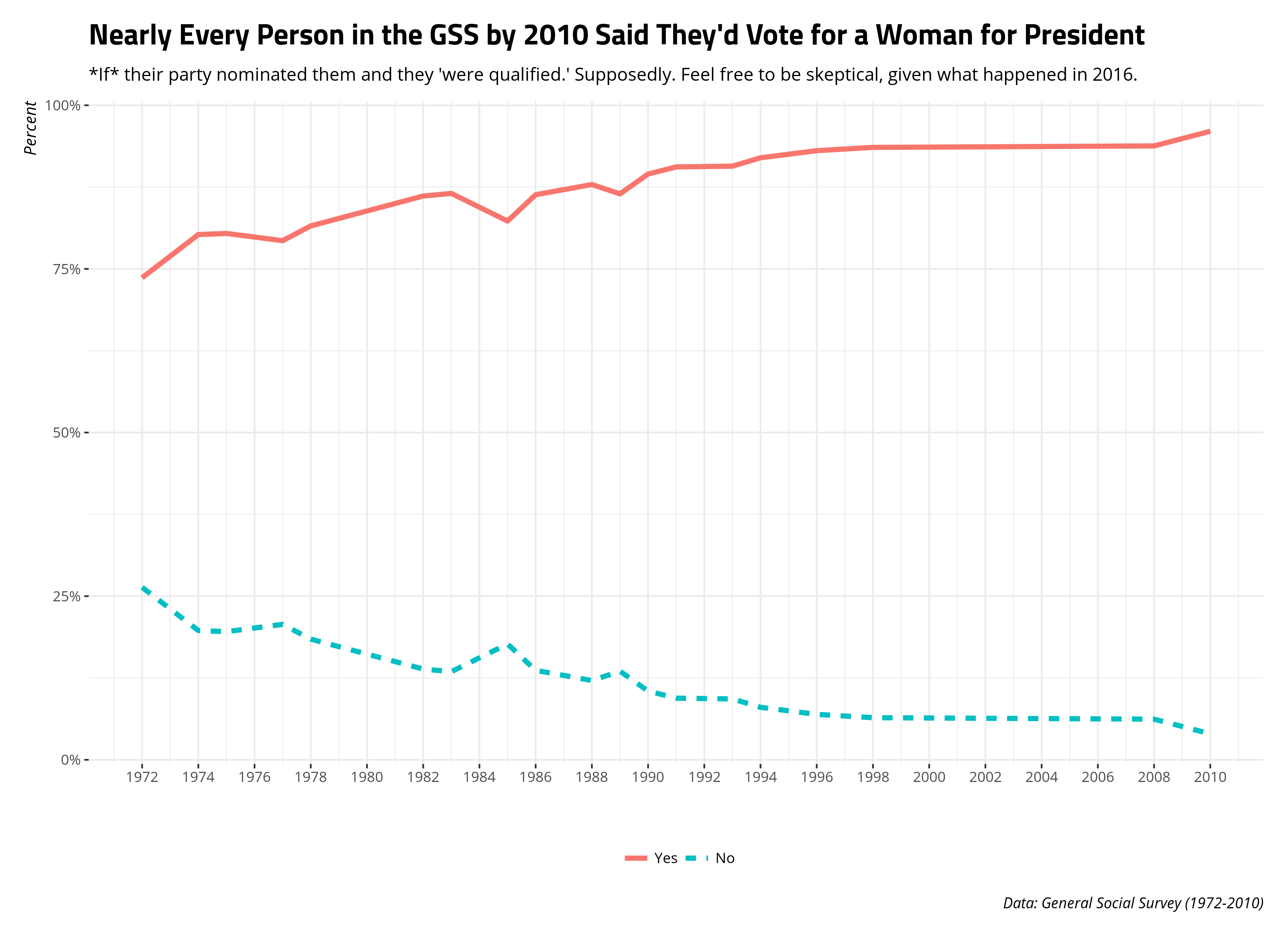
Helpfully, you can also use {dplyr} syntax to do even lazier queries. Here’s one example in the GSS data. The GSS has periodically asked its respondents this interesting question (fepres): “If your party nominated a woman for President, would you vote for her if she were qualified for the job?”. There is a lot to unpack here. It’s an interesting question to ask and, helpfully, the GSS made sure to qualify the question with “your party.” The GSS asked it in most survey waves between 1972 and 2010, but not since 2010. Let’s grab it. Let’s also grab the data for whether the respondent believes the United States is spending too little, about the right amount, or too much on highways and bridges (natroad). This was asked every survey year from 1984 to 2018. I’m not going to do anything with this data, but I’m going to use it to emphasize how lazy of a query you can do here thanks to {dplyr}.
all_years <- DBI::dbListTables(gsspgcon)

all_years %>%
  map(~{
    tbl(gsspgcon, .x) %>%
    select(one_of("year", "uid", "fepres", "natroad"))
  }) %>%
  reduce(function(x, y) union(x, y)) -> gss_query
This will produce warnings, but the use of one_of() in the select() function means the warnings will just advise you about data unavailability. We knew that would happen and did it by design. Here’s the ensuing output. Observe that the use of one_of() in select(), alongside other {dplyr} mechanics, just created NAs for cases where one of the two variables was not asked in one of the survey waves.
gss_query %>% arrange(year, uid)
#> # Source:     lazy query [?? x 4]
#> # Database:   postgres [steve@/var/run/postgresql:5432/gss]
#> # Ordered by: year, uid
#>     year   uid fepres natroad
#>    <dbl> <int>  <dbl>   <dbl>
#>  1  1972     1      1      NA
#>  2  1972     2      2      NA
#>  3  1972     3      1      NA
#>  4  1972     4      1      NA
#>  5  1972     5      1      NA
#>  6  1972     6      2      NA
#>  7  1972     7      1      NA
#>  8  1972     8      1      NA
#>  9  1972     9      1      NA
#> 10  1972    10      1      NA
#> # … with more rows
Likewise, when you’ve finished your query, use collect() to more fully use R’s functionality to do data analysis.
gss_query %>%
  collect() %>%
  # There are so few "wouldn't votes" (only 4 total in just two waves)
  # Let's ignore them
  mutate(feprescat = case_when(
    fepres == 1 ~ "Yes",
    fepres == 2 ~ "No"
  )) %>%
  mutate(feprescat = fct_relevel(feprescat, "Yes", "No")) %>%
  group_by(year, feprescat) %>%
  tally() %>% na.omit %>%
  group_by(year) %>%
  mutate(tot = sum(n),
         perc = n/tot)
The goal of this post is more about the method than the substance. Here’s how I’d recommend storing your wide/tedious-to-load data as tables in a relational database. {dplyr} and {purrr} can get a lot out of these databases with just a little bit of code and knowledge about the underlying data. There’s more I can/should do here (e.g. stripping out the “Inapplicables” as missing data in the GSS), but you may find this useful. It’s a smart way to store your bigger data sets in the social/political sciences so you can explore them as quickly and conveniently as possible. You can also learn a bit more about SQL syntax along the way.
When you’re done, remember to “disconnect” from the database.
DBI::dbDisconnect(wvspgcon)
DBI::dbDisconnect(gsspgcon)
-
The United States does not appear to be in the second survey wave provided in the six-wave WVS data. ↩
Disqus is great for comments/feedback but I had no idea it came with these gaudy ads.