Two Helpful R Markdown/Jekyll Tips for an Easier Blogging Experience

Jekyll rules the world. Your Jekyll friend, Steve

Last updated: May 04, 2022

It’s crazy to think I transitioned my website from Wordpress to Jekyll four years ago this month. About two and a half years ago (example), I started doing some R blogging by using the {servr} package to render some R Markdown-based analyses as blog posts.

The former experience (Jekyll) has been much easier than the latter experience (getting R Markdown to play nice with Jekyll). Basically, {servr} works as a wrapper for rendering a site in Jekyll, scanning a directory for some source R Markdown scripts and rendering them as blog posts. I’ve never had a great experience with it for two reasons. First, {servr} always struck me as clunky in approach and perhaps even clunkier in execution. It’s a great tool for compiling and rendering R Markdown files as a blog posts, but it seems like conceptual overkill when only a handful of my blog posts include analyses in R. I found the experience clunky as well. {servr} seemed to take more time building (“serving”) my website than a standard jekyll serve -w call in a terminal. It wanted to render any R Markdown file it could find rather than the one I wanted it to render, which raised the possibility of it breaking a post from a few years ago because of a package dependency issue that I may not have noticed emerge over the years. It would also choke, violently, on any error I committed in the document and take 30 seconds or so to reset after spamming the R console with errors. There has to be a better way!

I think I stumbled on two tips for a better blogging experience with Jekyll and R Markdown and thought sharing them here might help some others.

Manually Render R Markdown Posts with a Few Lines in YAML

It might be better to skip {servr} altogether and just manually compile your R Markdown posts to the _posts directory (where Jekyll stores blog posts by default). Just a few lines in the YAML will do it.

First, assume you store your R Markdown posts in a separate directory (typically _source, which is how I have it on my Github) and want to render them to the _posts directory. This is what the servr package does when it builds a Jekyll site. Toward that end, keep the R Markdown files in that _source directory but change your YAML to be someting like this (based on the post on which I’m working right now).

---
title: Two Helpful R Markdown/Jekyll Tips for an Easier Blogging Experience
output:
  md_document:
    variant: gfm
    preserve_yaml: TRUE
knit: (function(inputFile, encoding) {
  rmarkdown::render(inputFile, encoding = encoding, output_dir = "../_posts") })
author: "steve"
date: '2019-08-01'
excerpt: "Here are two tips for having what I think will be an easier blogging experience in R Markdown and Jekyll."
layout: post
categories:
  - R Markdown
  - Jekyll
image: brent-rambo.jpg # for open graph protocol
---

This looks like boilerplate YAML for any post on a Jekyll blog. It’s the output: and knit: fields I want to highlight here. First, I think it’s a better approach for my blogging workflow to just manually render a document as if I were rendering an academic paper. For this purpose, change the output to md_document:. The variant: gfm (Github-flavored markdown) is probably optional, but preserve_yaml: TRUE is not. Make sure to put that in there.

The knit: option is a convoluted way of specifying that the finished markdown document should be in the _posts directory. The relative path there (i.e. ../) says to backtrack one directory (i.e. from _source) to the root directory, and then go into the _posts directory.

I like this workflow better than using servr to build my blog. Here, I can build my site in terminal with jekyll serve -w and open up the preview version at http://localhost:4000, and use R Markdown to knit the R Markdown document as a blog post. From there, it’s a matter of clicking the link to the blog post in the browser and refreshing every time I update the R Markdown document to see what it looks like.

Alternatively: Just Knit it in the Console if You Have Some Jekyll Liquid Tags

The aforementioned setup should work for most people in most applications. However, most of my posts have a lead image that’s wrapped in a Jekyll Liquid tag. You can see what it does here. It basically calls in a few parameters to render an image like how my Wordpress installation used to do it.

<dl id="" class="wp-caption align{{include.align}}" style="max-width: {{include.width}}px">

<dt><a href="{{ include.href }}"><img class="" src="{{ include.url }}" alt="{{ include.caption }}" /></a></dt>

<dd>{{ include.caption }}</dd>
</dl>

This creates a problem for using R Markdown to render to a normal markdown document. For one, I know of no way to pass raw HTML through R Markdown to render it to a Markdown document. Further, R Markdown won’t correctly process Liquid tags either. It’d be nice if it ignored it, but it’ll try (and fail) to render it. In addition, a clever use of the results="asis" option with a cat() function will still lead to problems. Basically, it creates a quotation mark encoding issue in which standard “neutral” quotation marks get rendered as left and right quotation marks. That’ll break a Liquid tag; it seems.

There’s a workaround if you’re wanting to use Liquid tags in R Markdown posts. First, wrap the Liquid tag in an R Markdown chunk. Set eval=TRUE, echo=FALSE, and, importantly, results="asis". Thereafter, wrap it in a cat() command in R as I do for the lead image.

cat('{% include image.html url="/images/brent-rambo.gif" caption="Jekyll rules the world. Your Jekyll friend, Steve" width=410 align="right" %} ')

Then, just knit it and specify and output file in the _posts directory. It helps to set the working directory to the _source directory of the Jekyll blog before you do this.

setwd("~/Dropbox/svmiller.github.io/_source") # adjust to your preferences.
knitr::knit("2019-08-01-two-helpful-rmarkdown-jekyll-tips.Rmd",
            output = "../_posts/2019-08-01-two-helpful-rmarkdown-jekyll-tips.md")

The benefit of this approach is it skips R Markdown’s render function altogether. Plus, this approach means you can ignore the knit: field in the YAML. However, it does mean making sure you correctly spelled the output file. The silver lining here is typing out this command once means it’s in the console in Rstudio. Hitting up in the console will retrieve it from the session history so you don’t have to keep typing it out.

Tweak Where the R Graphs Are Stored

One problem I kept encountering in doing R Markdown blogging is the graphs I generated would never have the URLs I wanted them to have. I usually set a setup chunk with an option like knitr::opts_chunk$set(fig.path = '../images'). This saved the graphs where I wanted them to go (i.e. in the images directory on my blog) because the _source or _post directory shares the same directory as the images directory. However, the rendered post would have images with locations like http://svmiller.com/2019/08/images/image-name.png because of my custom permalinks when I wanted http://svmiller.com/images/image-name.png.

This too is an easy fix. For each of the R Markdown posts in the source directory, make a setup chunk at the top of the document (after the YAML). Set include=FALSE and cache=FALSE, Then add the following bits of code, per this post from Randi Griffin.

base_dir <- "~/Dropbox/svmiller.github.io/" # i.e. where the jekyll blog is on the hard drive.
base_url <- "/" # keep as is
fig_path <- "images/" # customize to heart's content, I 'spose.

knitr::opts_knit$set(base.dir = base_dir, base.url = base_url)
knitr::opts_chunk$set(fig.path = fig_path,
                      cache.path = '../cache/',
                      message=FALSE, warning=FALSE,
                      cache = TRUE) 

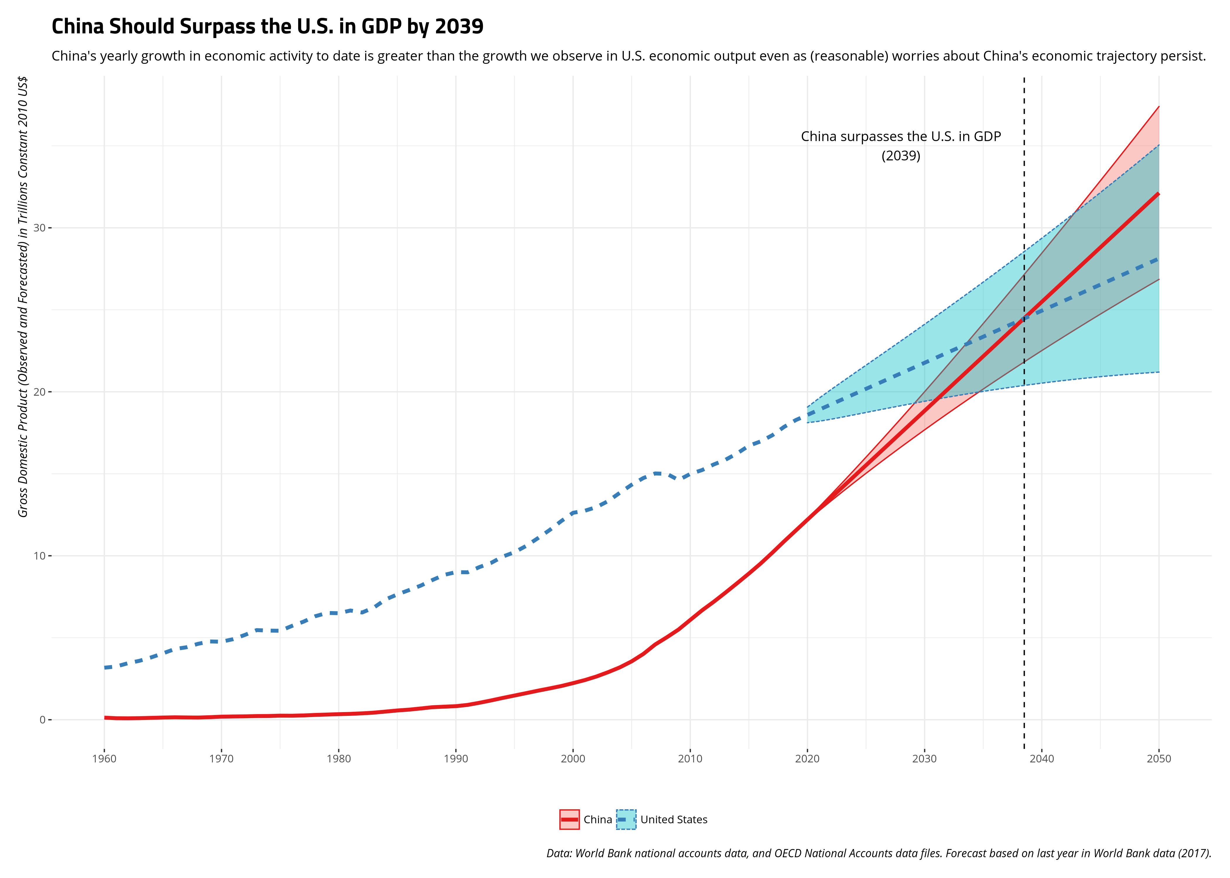
The R Markdown blogging workflow is much more straightforward after that. I can now seamlessly generate and display some graphs when I render the R Markdown document. For example, here is a graph on GDP forecasts I did and stored in my {stevedata} package as a data set. This is for an in-class lecture for my intro class on the future of international politics (in particular, the “Rise of China”).

usa_chn_gdp_forecasts %>% 
  mutate(gdp = ifelse(is.na(gdp), f_gdp, gdp)) %>%
  mutate(gdp = gdp/1e12,
         f_lo80 = f_lo80/1e12,
         f_hi80 = f_hi80/1e12) %>%
  ggplot(.,aes(year, gdp,  linetype=country, color = country, fill= country)) +
  theme_steve_web() +
  geom_ribbon(aes(ymin = f_lo80, ymax = f_hi80), alpha = 0.4) +
  geom_line(size=1.5) +
  scale_x_continuous(breaks = seq(1960, 2050, by = 10)) +
  xlab("") + ylab("Gross Domestic Product (Observed and Forecasted) in Trillions Constant 2010 US$") +
  geom_vline(xintercept = 2038.5,linetype = "dashed") +
  scale_color_brewer(palette = "Set1") +
  annotate("text", x=2028, y = 35, 
           label = "China surpasses the U.S. in GDP\n(2039)", 
           hjust = .5, family = "Open Sans")  +
  labs(title = "China Should Surpass the U.S. in GDP by 2039",
       fill = "", color = "", linetype = "",
       subtitle = "China's yearly growth in economic activity to date is greater than the growth we observe in U.S. economic output even as (reasonable) worries about China's economic trajectory persist.",
       caption = "Data: World Bank national accounts data, and OECD National Accounts data files. Forecast based on last year in World Bank data (2017).")