Learning About Expected Categorical Relations (Chi-Squared Tests) in R by Way of Arms Races and War

- An Eritrean soldier stands in front of a destroyed T-55A tank in 1999. This war starts in 1998 but the mutual military build-up for it arguably started in 1996. (Broń Pancerna/Flickr)
This is a post I’m writing just to spam material to my blog, and also to pad material I need to prepare for my IRIII students in their quantitative methods sequence. It’s a challenge to teach them stuff that is super basic, but has a real-world application, and in the limited time I have with them. The class had historically been built toward just getting them to do lm() in R (or regress in Stata) and to be happy if they can do that. However, there’s been some shuffling amid hour cuts that incidentally gives me more time to teach them more stuff. But, again, it has to be simple.
Enter the arms race and war debate. I cut my teeth on this debate in graduate school and still like to teach around the basics of this stuff when I can. I still think Lewis Fry Richardson’s linear theory of nations gets at the core of how we should conceptualize the arms race, acknowledging it’s a glorified port of his training in mathematics to the realm of international relations.1 Admittedly, it is a bit of a dated topic. Perhaps it’s fair to note that the “arms race” of a century or two ago looks nothing like what an arms race would resemble now. It won’t be simple expenditures. It won’t be manpower. It won’t even be boats. But the substance of this debate maps nicely to two thing I want to accomplish in an IR curriculum at the bachelor’s level. First, it highlights how a lot of realpolitik conventional wisdom stretches so thin it strains to cover anything in detail. Second, the empirical application of this debate is all chi-squared tests. There are definitely more advanced ways of approaching this, especially with what this means in the 21st century. But, you can learn about the chi-squared test with these things I’d have you read anyway if I could.
Here are the R packages I’ll be using today. Do note that {stevedata} has a forthcoming data set I’ll be using to offer another means to assess this relationship.
library(tidyverse)   # for my basic workflow
library(stevedata)   # forthcoming v. 1.7.0, for `mmb_war` data
library(stevethemes) # for themes
library(kableExtra)  # for tables

theme_set(theme_steve()) # setting a default theme
Here’s a table of contents.
Let’s get started.
The Debate: Para Bellum and the “Steps to War”
Si vis pacem, para bellum (if you want peace, prepare for war)
This aphorism sounds cool and, from a so-called “realist” worldview, it has a certain kind of logic by which it works. Intuitively, a true balance of power between two states in which neither side could comfortably defeat the other side makes war an unattractive option. It’s the same kind of logic that underpins mutual assured destruction. It may not sound pleasant to the pacifist, but “peace through strength” is sound strategy if you were to think of it in this particular way. Mutual military build-ups evoke certain tensions or anxiety in the general public about an impending war, though the behavior itself would be perfectly rational if the idea is to avoid war. A rational state substantially increases it might to prepare for war, wanting peace. A rival state requites that militarization/mobilization, preparing for war while wanting peace. Together, they achieve an equilibrium where an increased mobilization for war makes peace more attractive than it might have been in the absence of the mutual build-up. So that story goes.
There is a group of us in international relations that have always found this, at best, laughably simplistic and, more to the point, a ridiculous proposition of an equilibrium. Richardson’s work is foundational on this topic, though perhaps it’s fair to say his conclusions are importantly conditioned by his own pacifist ideals. J. David Singer (1958) started his article with that exact quote, as relayed by Vegetius, and noted the immediate epilogue under Theodosius I was a spate of violence conducted by the emperor.2 My training is largely in the “Steps to War” tradition of John Vasquez. There are underlying causes of war (prominently the allocation of territory) and proximate causes (“steps”) of war. Violence is not unique to humans, but warfare arguably is a unique kind of learned, social behavior. Realpolitik policy prescriptions (like arms races) prepare states for sustained combat and only heighten mistrust of the other side under what was already less than rosy conditions. The “steps” policymakers take under those circumstances limit future options, forgo more peaceful off-ramps, and further empower domestic “hardliners” or “hawks” to favor further aggression. Another way of thinking about this is to ask why you’re arms-racing in the first place. Why are you? Certainly not because things are going great and certainly not because no one with power/influence in society wants to use these toys. Be real, so-called “realists.”
The Empirical Debate Between Wallace (1979) and His Critics
The empirical debate on this relationship may not have started with Wallace (1979), but it sure as heck escalated under him. His Table 2 (reproduced below) argued arms races almost always lead to war (23 occurrences to five non-occurrences) and the absence of arms races almost never lead to war (three wars in the absence of arms races to 68 non-wars). For those who like working with percentages, that’s a comparison of 82% to 4% for 99 total cases. It’s more than enough to suggest something is happening here.
| Arms Race | No Arms Race | |
|---|---|---|
| War | 23 | 3 |
| No War | 5 | 68 |
However, there are several important reasons to doubt how Wallace came to this conclusion.3 Critiques came in all directions for this analysis, including Altfield (1983), Horn (1987), Morrow (1989), and Weede (1980) (among many others, I’m sure). I want to focus on Diehl (1983) as largely capturing all the recurring themes in this critique of Wallace (1979). Namely: Wallace is describing a measure of arms races that he never makes publicly available and could not replicate. It’d be difficult to know for sure, but his polynomial arms race function he describes would also inadvertently pick up unilateral buildups. Further, it’s pretty clear that the world wars are the lion’s share of his empirical support. He’s additionally compounding this problem by disaggregating all of them (even if there is an ongoing war, like his USSR-Japan case in 1945). In one re-analysis of this relationship (Table II), Diehl reports the relationship between arms races and war is basically a null relationship. Three of 13 arms races lead to war (23%) compared to a nine wars in 73 cases (12%) not preceded by an arms race. One rate is more than the other, but it’s not a discernible relationship. There is no clear relationship by which arms races lead to war.4
| Arms Race | No Arms Race | |
|---|---|---|
| War | 3 | 9 |
| No War | 10 | 64 |
| Note: Chi-sq: 1.06, n = 86. |
When I do get the opportunity to teach about arms races, I offer Susan Sample (1997) as a kind of Solomon in this debate. The empirical debate employed multiple different operationalizations of arms races and multiple different dispute data sets. A battery of analyses mix-and-matching different data sets yields the overall conclusion that arms races are positively associated with dispute escalation to war, even if it’s fair to note Wallace’s (1979) original conclusions were far too stark. See, as just one example, her Table IX using Diehl’s arms race index with all major state militarized interstate disputes. 14 of the 53 disputes in which there was an arms race led to war (26%). Just 17 of the 204 (8%) of the disputes in which there wasn’t an arms race led to war. That is a discernible difference, if clearly not the magnitude difference originally reported by Wallace (1979).
| Arms Race | No Arms Race | |
|---|---|---|
| War | 14 | 17 |
| No War | 39 | 187 |
| Note: Chi-sq: 13.0, n = 257. |
I’ve glossed over to this point the exact tests scholars were using in this debate over operationalization and sample selection. It’s almost always a chi-squared test of independence for observed and expected counts. You could actually do this yourself with no real effort at all to understand the inferential claims the various people in this debate are making.
The Chi-Squared Test
Chi-squared (\(\chi^2\)) tests are common tests to use in very basic applications to assess whether the observed counts in some kind of category for two (or more) groups are discernibly different than what would be expected if there were no difference between or among the groups. It’s easier to introduce students to this in a simple 2x2 application like this and it will lean on the contingency tables you’ve seen everywhere to this point.
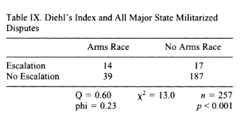
- Table IX (Sample, 1997)
First, let’s show Sample’s (1997) actual Table IX to see what’s happening here. Notice the 2x2 contingency table reproduced above. The primary grouping variable here is in the column whereas the rows are a kind of outcome of interest to us (war or no war). Let’s further calculate some total information about the data. There are 31 wars (14 with arms races, 17 without them). There are 226 disputes in the data that did not escalate to war (39 with arms races, 187 without them). Those are our row totals. We noted the column totals above. There were 53 disputes with arms races preceding them in these data (14 of which became wars). There were 204 disputes without arms races preceding them (17 of them escalating to war). Let’s expand this table a bit with this information.
| Arms Race | No Arms Race | Row Total | |
|---|---|---|---|
| War | 14 | 17 | 31 |
| No War | 39 | 187 | 226 |
| Column Total | 53 | 204 | 257 |
We next need to calculate expected counts, or what we would expect if there were no association between arms races and war. Formally, each expected value in a given cell is equal to the row total times the column total, divided over the total number of observations (257, in all cases).
| Arms Race | No Arms Race | |
|---|---|---|
| War | (31*53)/257 = 6.393 | (31*204)/257 = 24.607 |
| No War | (226*53)/257 = 46.607 | (226*204)*257 = 179.393 |
The formula for the chi-squared test statistic is very straightforward. It’s something you could do on paper, or in Excel even. It would take more effort, but it’s not difficult at all.
\[\chi^2 = \sum \frac{(O - E)^2}{E}\]For all cells in the contingency table, take the difference between observed and expected count, square it, divide it over the expected count, and add them all together. That’s your chi-squared statistic. In our case, that produces a chi-squared statistic of about 12.965.
| Arms Race | No Arms Race | |
|---|---|---|
| War | (14 - 6.393)^2/(6.393) = 9.051 | (17 - 24.607)^2/(24.607) = 2.351 |
| No War | (39 - 46.607)^2/(46.607) = 1.241 | (187 - 179.393)^2/(179.393) = .322 |
We could also check our work by doing it in R. Notice we’re going to capture the chi-squared statistic that Sample (1997) reported in her Table IX, give or take some rounding for presentation.
etl <- (31*53)/257
ebl <- (226*53)/257
etr <- (31*204)/257
ebr <- (226*204)/257

etl; ebl; etr; ebr
#> [1] 6.392996
#> [1] 46.607
#> [1] 24.607
#> [1] 179.393

csctl <- (14 - etl)^2/(etl)
cscbl <- (39 - ebl)^2/(ebl)
csctr <- (17 - etr)^2/(etr)
cscbr <- (187 - ebr)^2/(ebr)

csctl; cscbl; csctr; cscbr
#> [1] 9.051548
#> [1] 1.241584
#> [1] 2.351628
#> [1] 0.3225684

chisq <- csctl + cscbl + csctr + cscbr

chisq # rounding above is off 2/1000ths or so, but that's no biggie.
#> [1] 12.96733
We’re not quite done yet because we need to relate this test statistic to what we might expect to observe under some kind of distribution. So-called the chi-squared test, the test statistic is related to the chi-squared distribution. The chi-squared distribution is a unique distribution of the sum of squared standard normal variables with just a single parameter: the degrees of freedom. It determines the number of independent standard normal variables to sum. For a single degree of freedom, this distribution will have a clear right tail. More degrees of freedom result in distributions that look more “normal.” Observe:
set.seed(8675309) # Jenny, I got your number...

nobs <- 10000
tibble(`rchisq(df = 1)` = rchisq(nobs, df = 1),
       `rchisq(df = 2)` = rchisq(nobs, df = 2),
       `rchisq(df = 5)` = rchisq(nobs, df = 5),
       `rchisq(df = 10)` = rchisq(nobs, df = 10),
       `rchisq(df = 25)` = rchisq(nobs, df = 25),
       `rchisq(df = 50)` = rchisq(nobs, df = 50))
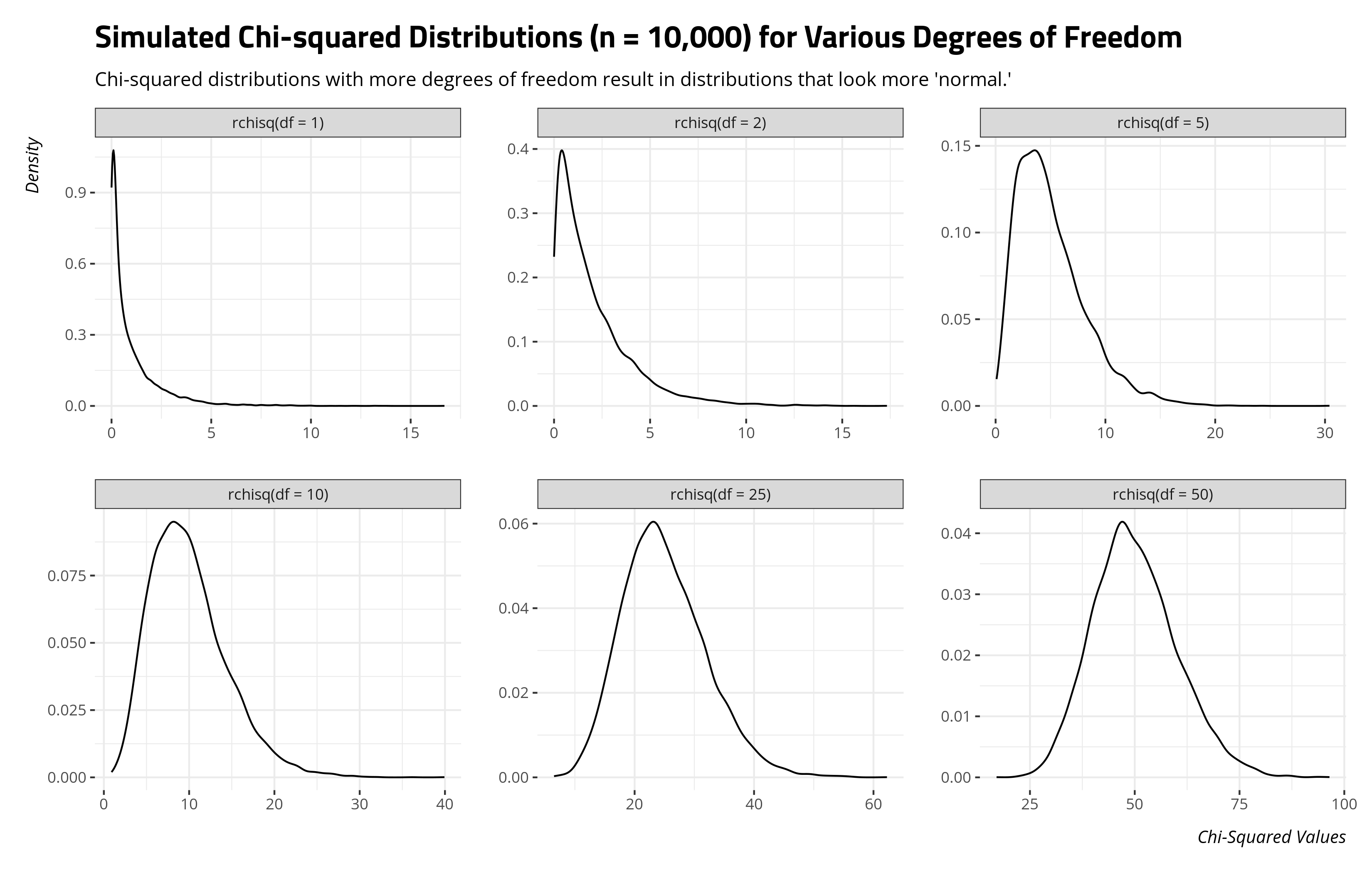
In the case of the chi-squared test, the degrees of freedom is equal to the product of the number of rows (minus 1) and the number of columns (minus 1). For a simple 2x2 contingency table, that’s 1. Inference here works in the same way it does most other applications. Higher test values (lower p-values) will indicate greater incompatibility with the distribution, suggesting a rejection of the null hypothesis of no association. You can do this in R with the pchisq() function.
pchisq(chisq, df = 1, lower.tail = F)
#> [1] 0.0003169742
Or, better yet, just do all this in R with the chisq.test() function. The only real headache with this is you’ll have to teach yourself how to deal with matrices in R since that’s what the chisq.test() function generally wants.5 Here’s how you do it without Yates’ continuity correction (correct = FALSE), which is what these analyses were doing.6
# The observed counts, as a single vector
c(14, 39, 17, 187)
#> [1]  14  39  17 187
# In matrix form, using nrow = 2. When doing it this way, R files column by
# column. That means the first column gets the first two values, which is
# incidentally what we want. There are other ways of doing this, though.
matrix(c(14, 39, 17, 187), nrow = 2)
#>      [,1] [,2]
#> [1,]   14   17
#> [2,]   39  187

# Chi-squared test with*out* continuity correction.
chisq.test(matrix(c(17, 187, 14, 39), nrow = 2), correct = FALSE)
#>
#> 	Pearson's Chi-squared test
#>
#> data:  matrix(c(17, 187, 14, 39), nrow = 2)
#> X-squared = 12.967, df = 1, p-value = 0.000317
A Re-Analysis Using Newer Data
mmb_war is in the forthcoming version 1.7.0 of {stevedata} and offers a re-analysis of this using newer data. Here’s a glimpse into the data here.
Data <- mmb_war
Data
#> # A tibble: 2,324 × 9
#>    ccode1 ccode2 tssr_id micnum  year dyfatmin dyfatmax sumevents   mmb
#>     <dbl>  <dbl>   <int>  <dbl> <dbl>    <dbl>    <dbl>     <dbl> <dbl>
#>  1      2     40     130    246  1960        0        0        20     0
#>  2      2     40     130     61  1962        0        0        35     0
#>  3      2     40     130   2225  1979        0        0         2     0
#>  4      2     40     130   2972  1981        0        0         4     0
#>  5      2     40     130   2981  1983        0        0         1     0
#>  6      2     40     130   3058  1983        4       25         2     0
#>  7      2     40     130   2742  1986        0        0         2     0
#>  8      2     70      32   1554  1836        0        0         5     0
#>  9      2     70      32   1553  1838        0        0         4     0
#> 10      2     70      32   1556  1839        0        0         2     0
#> # ℹ 2,314 more rows
I take inspiration from Gibler et al.’s (2005) analysis on arms races and war and follow their lead in recreating a data set on arms races that I merge into this data set on all dyadic confrontations among strategic rivals.7 Importantly, I’m looking for whether there was a mutual military build-up that started and was ongoing prior to the start of the confrontation, in addition to whether the confrontation in question escalated to the point of dyadic war (i.e. whether the minimum dyadic fatalities surpassed 1,000).
First, let’s create a war measure that equals 1 if the minimum dyadic fatalities surpassed 1,000.
Data %>% mutate(war = ifelse(dyfatmin >= 1000, 1, 0)) -> Data
Now, let’s create a contingency table of the mutual military build-ups and the dyadic war.
table(Data$war, Data$mmb)
#>
#>        0    1
#>   0 2049   75
#>   1  180   20
Invoking the table() function here with 0s and 1s is a bit clumsy for what I want, but should be read as follows. The row labels of 0 (no war) and 1 (war) relate to the first vector (i.e. the war dummy). The column labels of 0 (no mutual military build-up) and 1 (mutual military build-up) relate to the column labels of the mutual military build-up dummy variable. If we flip things around a bit, we’d note that 20 of the 95 observations of dyadic confrontations succeeding mutual military build-ups reuslted in war (21%). 180 of the 2,229 dyadic confrontations without a mutual military build-up preceding them reached fatality thresholds we could classify as a war. That’s about 8%. It looks like a significant difference, but we’d have to see what the chi-squared test says.
# Chi-squared test with continuity correction.
# Fyi: you could read in the vector to matrix() as c(2049, 180, 75, 20) and it'd
# be the same thing. I just prefer to see it this way.
chisq.test(matrix(c(20, 75, 180, 2049), nrow = 2), correct = TRUE)
#>
#> 	Pearson's Chi-squared test with Yates' continuity correction
#>
#> data:  matrix(c(20, 75, 180, 2049), nrow = 2)
#> X-squared = 17.895, df = 1, p-value = 2.335e-05
If there were no association between the arms races and war, the divergence between what’s observed and what we’d expect results in a chi-squared statistic so wildly incompatible with what we’d expect for a chi-squared distribution with a single degree of freedom. We reject the null hypothesis of no association and instead suggest the results are more compatible with an association between arms races and escalation to war.
Conclusion
This is mostly for the kids to give them something to do in a lab session for quantitative methods. It’d be nice for students in my program to get more of the boilerplate quantitative peace science stuff that I got in grdauate school. It would be nice for them to further contextualize why a lot of so-called “realist” talking points are poorly stated. It’d be nice for them understand more of John Vasquez. It would further be great to get them to do stuff in the R programming language. This particular application offers all of that. There are more advanced ways of doing this, and it asks a lot for logics derived from observations of boats (or even nuclear weapons) to map to the current system. Still, it’s classic stuff with classic methods. Students should know this stuff anyway.
-
It’s a system of linear equations! It’s an elementary way of thinking about it but does well to represent the phenomenon in a basic form. ↩
-
Dating the tract from which the “Para Bellum” quote originates is tricky and it’s conceivable Singer is referring to what might be understood in modern terminology as “intra-state” or “extra-state” violence. Certainly, the Roman Empire of this time precedes the modern state system. No matter, it shouldn’t be lost on the reader that this would still mean an emperor mobilized a bunch of hammers and now needs to find nails somewhere. The relationship between external threat and non-democracy is quite robust. Such a mobilization makes state-sanctioned violence cheaper than it would be in the absence of such a mobilization. ↩
-
Brandon Valeriano, may he rest in peace, told me once about a conversation he had with Wallace about the operational details of his analysis and how exactly he arrived at such stark conclusions in an era of punch-card analyses. It’s informative but I don’t think I can share them here. Wallace passed away in 2011. ↩
-
It is interesting that a lot of the empirical critiques of Wallace mostly (and rightly) say Wallace was way off what the true relationship is, but don’t really vindicate the “para bellum” hypothesis that they should lead to peace. ↩
-
The operative arguments you’ll want to learn are
nrow,ncol, andbyrow. Observe, for example, the difference betweenmatrix(c(1:4), nrow = 2)andmatrix(c(1:4), nrow = 2, byrow=TRUE)for a simple 2x2 matrix. Be mindful that the chi-squared test is agnostic about what are rows and what are columns because it largely hinges on the multiplication of row totals and column totals. Transposing a matrix would result in equal chi-squared statistics (e.g.chisq.test(t(matrix(c(1:6), ncol = 2)))andchisq.test(matrix(c(1:6), ncol = 2))). I work on the convention from Pollock III (2016) that things informally understood as “causes” should be columns and things informally understood as “outcomes” should be rows in creating a cross-tabulation like this. In our case, war is understood as an outcome of arms races. However, the particular method here has the same limitations as Pearson’s r. Use it with that in mind. ↩ -
R’s default behavior sets Yates’ default continuity correction to TRUE. This is the more conservative approach to a chi-squared test statistic because it will generally push down the test statistic for smaller samples to avoid Type I errors. ↩
-
You can see the details section of the codebook for a conversation about some case exclusion rules I employed along the way. I’m still tinkering with this military build-up measure and do not offer it here to be used uncritically. ↩
Disqus is great for comments/feedback but I had no idea it came with these gaudy ads.