How Should You Think About Your Priors for a Bayesian Analysis?
- The intuition behind Bayesian inference.
There are any number of sticking points for a beginner to learning Bayes. For me, it was mostly about implementation. I’ll confess to being thrown for a loop about Markov chains before I got Jeff Gill’s math book in the summer of 2009 and spent some time on his treatment of that topic, but I mostly struggled with the software of the time that did not seem intuitive to me. {brms} has been integral toward increasing my pivot toward Bayes.
For the pure beginners, I think it’s the idea of specifying prior distributions. It’s certainly what just about every beginner text on Bayes I’ve seen spends the most time discussing. For beginners, the idea of prior expectations weighting the observed data to produce posterior distributions seems weird. It may even seem like it’s borrowing trouble. Bayesian inference is “subjective”, which is as much a design feature as it is a pejorative for dismissing the enterprise outright. A discomfort with the idea of prior distributions comes with a question of whether they are necessary. After all, if you elect to begin agnostic, and you have lots of data with which to play, the posterior is going to more closely resemble what the likelihood function communicates. You can have some really strong priors, but a fair bit of data at hand produces an ensuing posterior distribution that is going to map closely with the likelihood function. The extent to which prior distributions are sine qua non features of a Bayesian analysis, they are kind of problematic for newbies after their first semester or two of quantitative methods. Thus, if it may not matter much to inferences if you have plenty of data to use, do you need Bayes in the first place?
This post won’t answer that question1, but it will address the question/misgiving that precedes it: what do you do with prior distributions and how should you think about them? If you have like 10,000 observations with no real complex grouping structures in a boilerplate linear model, you don’t have to think hard about your prior distributions. It doesn’t mean you shouldn’t, just that your investment into understanding the nature of the data and your expectations from it will (probably) be swallowed by the observed data. However, if you have weaker/smaller data sets, those priors can matter a lot. That’s the situation I’ll be using in this post.
First, here are the R packages I’ll be using. I’ll only note here that CmdStan is my default engine for Stan and thank heavens that {brms} interfaces with it. Check it out. The speed upgrade is phenomenal.
library(tidyverse) # for all things workflow
library(stevemisc) # my toy R package, mostly for helper functions and plotting prettiness
library(stevedata) # for data
library(brms) # for Bayes stuff
library(tidybayes) # for additional Bayes stuff
library(kableExtra) # for tables
And here’s a table contents.
- First, the Boldest: the “Cocksure” Prior
- “Lazy” Normal Priors
- Have
{brms}Think of Priors For You - Have
{rstanarm}Think of Priors For You - Think of Your Own “Reasonable Ignorance” Priors
- What Different Priors Can Do to Our Inferences
- Conclusion: How Should You Think About Your Priors?
I’ll only add that Bayes can be a bit time-consuming, so a lot what I’m doing has been pre-processed. You can see the script here.
First, the Boldest: the “Cocksure” Prior
Most Bayesian texts I’ve read treat what follows here 1) last, if they address it at all, 2) technically not pure Bayesian if you’re peeking into your data to get some preliminary information for your prior expectations, and 3) only situationally a good idea. That said, “only situationally a good idea” is my middle name and this is an itch I’ve been wanting to scratch for a while.
Around this time last year, I wrote this guide on how to understand a linear regression model. The reviews were well-received. I’ve even been invited to present this to students in the United Kingdom (if remotely), hence the subject matter. It may not be immediately evident, but scroll down to that regression table. Therein, the unemployed variable, a dummy variable that equals 1 if the respondent is not currently employed but is actively looking for work, has a coefficient that is dwarfed by the standard error. Nothing looking like an issue from that at the onset; some variables just have really diffuse standard errors. However, a descriptive statistics table from the variables in that model points to a potential problem. You can check the _rmd directory on my website for the underlying code here as I typically hide code that results in tables (for web readability).
| Variable | Mean | Std. Dev. | Median | Min. | Max. | N |
|---|---|---|---|---|---|---|
| Age | 53.673 | 18.393 | 55 | 15 | 90 | 1893 |
| Education (in Years) | 14.049 | 3.631 | 13 | 3 | 41 | 1893 |
| Female | 0.541 | 0.498 | 1 | 0 | 1 | 1905 |
| Household Income (Deciles) | 5.171 | 2.973 | 5 | 1 | 10 | 1615 |
| Ideology (L to R) | 4.961 | 1.946 | 5 | 0 | 10 | 1726 |
| Pro-Immigration Sentiment | 16.891 | 6.992 | 17 | 0 | 30 | 1850 |
| Unemployed | 0.020 | 0.003 | 0 | 0 | 1 | 1905 |
Something looks amiss here in that unemployed variable. The mean of the dummy variable is about .02 (rounded) for a variable with 1,905 valid observations. This is because there are just 38 people in the entire data set who said they were unemployed but looking for work. That’s not a lot of information and that, perhaps more than anything, is why the regression model was unable to discern an effect of being unemployed on pro-immigration sentiment in the survey data I cobbled from the European Social Survey in 2018.
While we should note the data should be matched before doing something with inferential implications like this, the t-test suggests a potential difference in the means between both groups. On average, the unemployed are about 2.12 points lower in their pro-immigration sentiment than the gainfully employed or those not looking for active employment (e.g. housewives, students).
ttest_uempl <- t.test(immigsent ~ uempla, data=ESS9GB)
# be mindful of the direction here when you tidy up your t-test.
broom::tidy(ttest_uempl) %>%
  select(estimate:p.value)
#> # A tibble: 1 × 5
#>   estimate estimate1 estimate2 statistic p.value
#>      <dbl>     <dbl>     <dbl>     <dbl>   <dbl>
#> 1     2.12      16.9      14.8      1.68   0.102
# extract the standard error
round(as.vector(abs(diff(ttest_uempl$estimate)/ttest_uempl$statistic)), 2)
#> [1] 1.26
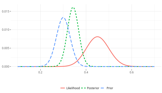
So, what if we were so sure—cocksure, even—that the true effect of being unemployed is to lower estimated pro-immigration sentiment by 2.12 points? Here, we believe this is the true effect and our regression model is not picking this up even though the t-test is. If we were so sure about this, we could specify this as a prior distribution on the estimated coefficient for unemployment with a normal distribution plugging in that difference in means as the mean of the distribution and the standard error of the t-test as the standard deviation of that distribution. I could obviously elect to be cocksure about more priors, but I really want to focus on just this one because it’s a unique data issue that the other variables don’t have.
With this in mind, a Bayesian approach leads to an interesting question not unlike the application in the Western and Jackman (1994) case. Here: what is the difference in what I can say about the effect of being unemployed on pro-immigration sentiment if 1) I really had no idea what the effect could be versus 2) I was so cocksure about what the t-test said?
# default/flat, don't-know-nothing priors
B0 <- brm(immigsent ~ agea + female + eduyrs + uempla + hinctnta + lrscale,
          data = ESS9GB,
          seed = 8675309,
          family = gaussian())

# cocksure prior, just for unemployment
cocksure_prior <- c(set_prior("normal(-2.12,1.26)", class="b", coef="uempla"))

B1 <- brm(immigsent ~ agea + female + eduyrs + uempla + hinctnta + lrscale,
          data = ESS9GB,
          seed = 8675309,
          prior = cocksure_prior,
          family = gaussian())
In a peculiar situation like this, the choice of a prior matters a great deal. With just 38 people reporting they are unemployed, there is not a lot of information about the effect of that variable on pro-immigration sentiment even if our data are reasonably powered (n = 1454). Were I to begin completely agnostic with default/flat priors, the effect leans negative but with diffuse standard errors capturing the poor quality of information for that variable. Were I to begin cocksure about the effect of being unemployed, the poor quality of information about the unemployed I have leads to an estimate that may not be as cocksure as the assumed prior effect, but is still more sanguine about the effect of being unemployed than if I were to begin completely agnostic. This has important inferential implications if I were exploring this question from the perspective of garden-variety null hypothesis testing.
I should offer a few comments about this approach. First, it’s technically cheating in the Bayesian framework. I’m using a t-test to get an informative prior and plugging it into the analysis. You should think about the prior distributions of your model before peeking at the data. That said, you can conjure a hypothetical situation where 1) past studies had shown that effect of being unemployed as having a mean of -2.12 with a standard deviation of 1.26 but 2) this particular data-generating process did not grab a lot of information on that particular variable. While this is technically cheating in this particular application, you could conjure a situation where it amounts to testing newer observations against a counterargument or conventional wisdom. Second, I’m calling this a “cocksure” prior just to be tongue-in-cheek. Bayesians would call this is a “strong prior”, and it is. However, if there is some stake attached to this particular coefficient for one reason or the other—perhaps you’re testing the political economy of immigration opinion framework like I did in this publication—be prepared to futz with that prior further. Explore how sensitive your inferences are to that prior distribution because, spoiler alert, they are in this case. They likely will be in your case if you encounter a situation like this.
“Lazy” Normal Priors
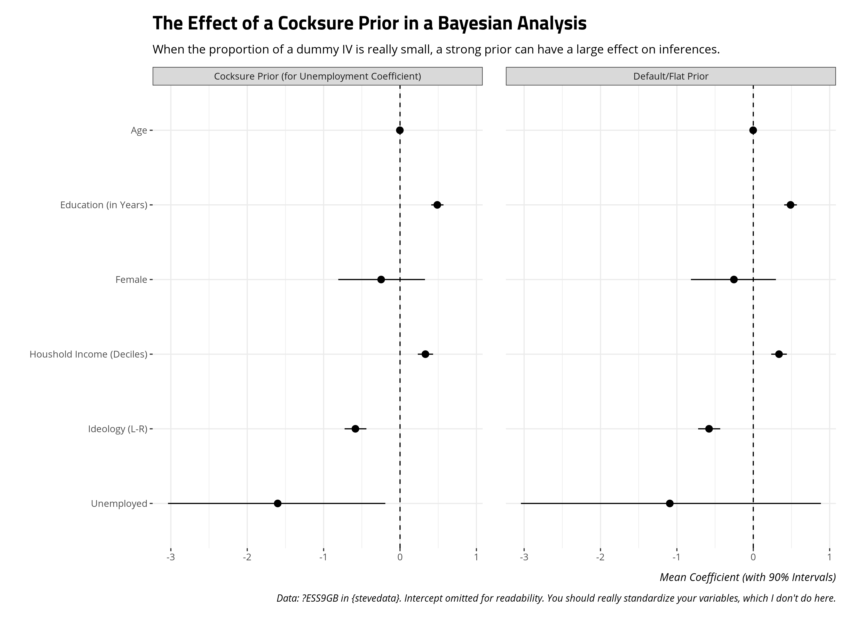
I think one of the oldest approaches to modeling prior distributions is to not think about them much at all. Western and Jackman’s (1994) approach to prior distributions is to just slap the most conceivably diffuse normal distribution on every parameter in the model (that didn’t have a strong prior attached to them in their particular application of competitive hypothesis-testing). Read a lot of empirically-oriented Bayesian analyses in political science and you’ll see some family of the normal distribution slapped onto model parameters. This can range from the standard normal distribution with a mean of 0 and a standard deviation of 1 (e.g. Gill and Witko, 2013) to the comically diffuse normal distribution with a mean of 0 and a standard deviation of 1,000,000 (e.g. Western and Jackman, 1994). I like how Gelman describes these. Standard normal is a “generic weakly informative prior” while the normal distribution with a standard deviation of 1,000,000 is a “super-vague” prior.
Let’s think of what this means in the context of the union density analysis, mostly because it’s a simple data set and Bayesian analyses can be time-consuming. Here, we’re trying to explain variation in the percentage of the workforce (employed or unemployed) that are union members between 1975 and 1980 as a function of the extent to which left-wing parties have controlled the government since 1919, the natural logarithm of the size of the labor force, and the concentration of employment, shipment, or production in industry. We’re going to use some family of a linear model, for which the important model parameters will be 1) the y-intercept, 2) the regression coefficients for those three independent variables, and 3) the residual standard deviation of the linear model.
The extent to which we know we want a linear model and that’s it and elect to not really think about the data or model further, we’re assuming those parameters could look something like this.
There are reasons you should choose to be careful here with this approach. Basically, these are lazy priors, one a little diffuse and the other really diffuse. You’re not really investing time into thinking about your data. No matter, one prevailing assumption in the statistics world is that things are distributed somewhat normally around some central tendency with observations further from it being less common. If you elect to begin agnostic about your parameters, prominently your regression coefficients, you’re starting at zero and assume the effect could plausibly be as large (positive or negative) as 2.5 (i.e. about 99% of the distribution in standard normal) or 2,500,000 (in the more comically diffuse distribution). These are ultimately lazy priors, but accessible for beginners who may at least know about the normal distribution.
In {brms}, you’d specify such prior distributions in our union density as follows.
brmform <- bf(union ~ left + size + concen)

lazy_priors_normal <- c(set_prior("normal(0,1)", class = "b", coef= "left"),
                         set_prior("normal(0,1)", class = "b", coef="size"),
                         set_prior("normal(0,1)", class="b", coef="concen"),
                         set_prior("normal(0,1)", class="Intercept"),
                         set_prior("normal(0,1)", class="sigma"))

lazy_priors_vague <- c(set_prior("normal(0,10^6)", class = "b", coef= "left"),
                         set_prior("normal(0,10^6)", class = "b", coef="size"),
                         set_prior("normal(0,10^6)", class="b", coef="concen"),
                         set_prior("normal(0,10^6)", class="Intercept"),
                         set_prior("normal(0, 10^6)", class="sigma"))
Have {brms} Think of Priors For You
Another alternative to thinking of your priors is to have some software package of choice think of them for you. It sounds bad when I say it that way, but let he who is without sin cast the first stone. My transition to more Bayesian approaches to inference came with some hand-holding, especially by {brms}.
The approach to default priors in {brms} seems to have changed over time—i.e. I remember seeing a lot of Student’s t with three degrees of freedom, a mu of zero, and a sigma of 10 when I started—but this appears to be how {brms} does it now. Because you the user are electing to have {brms} think of your priors for you, {brms} has little recourse but to look at your data to think of some reasonable areas for the sampler to explore. In the absence of specified priors for the regression coefficients, {brms} will slap on “improper flat priors.” These seem to amount to “no prior” even as the package’s author thinks of them as priors that are designed to influence the results as little as possible.
For a simple linear model, the other parameters get a Student’s t distribution that is going to lean on {brms} scanning the dependent variable. If the median absolute deviation of the dependent variable is less than 2.5, the sigma it chooses is going to be 2.5. If the median absolute deviation of the dependent variable is greater than 2.5, it will round that to a single decimal point and use that as the sigma. The Student’s t distribution that emerges for the y-intercept is going to have three degrees of freedom, a mu that equals the median of the dependent variable, and that sigma it selects. The residual standard deviation of the linear model is going to have a Student’s t with three degrees of freedom, a mu of zero, and that sigma it selects. Observe:
uniondensity %>%
  summarize(median_y = median(union),
            mad_y = mad(union)) %>%
  # There's assuredly a rounding issue happening here
  # but the principle is still clear
  data.frame %>%
  mutate_all(~round(.,2))
#>   median_y mad_y
#> 1    55.15 25.35

get_prior(brmform, data=uniondensity)
#>                     prior     class   coef group resp dpar nlpar lb ub
#>                    (flat)         b
#>                    (flat)         b concen
#>                    (flat)         b   left
#>                    (flat)         b   size
#>  student_t(3, 55.1, 25.4) Intercept
#>     student_t(3, 0, 25.4)     sigma                               0
#>        source
#>       default
#>  (vectorized)
#>  (vectorized)
#>  (vectorized)
#>       default
#>       default
Knowing well that a residual standard deviation of a linear model must always be positive, Bayesians describe such a prior on the sigma here as a “half-t” or words to that effect.
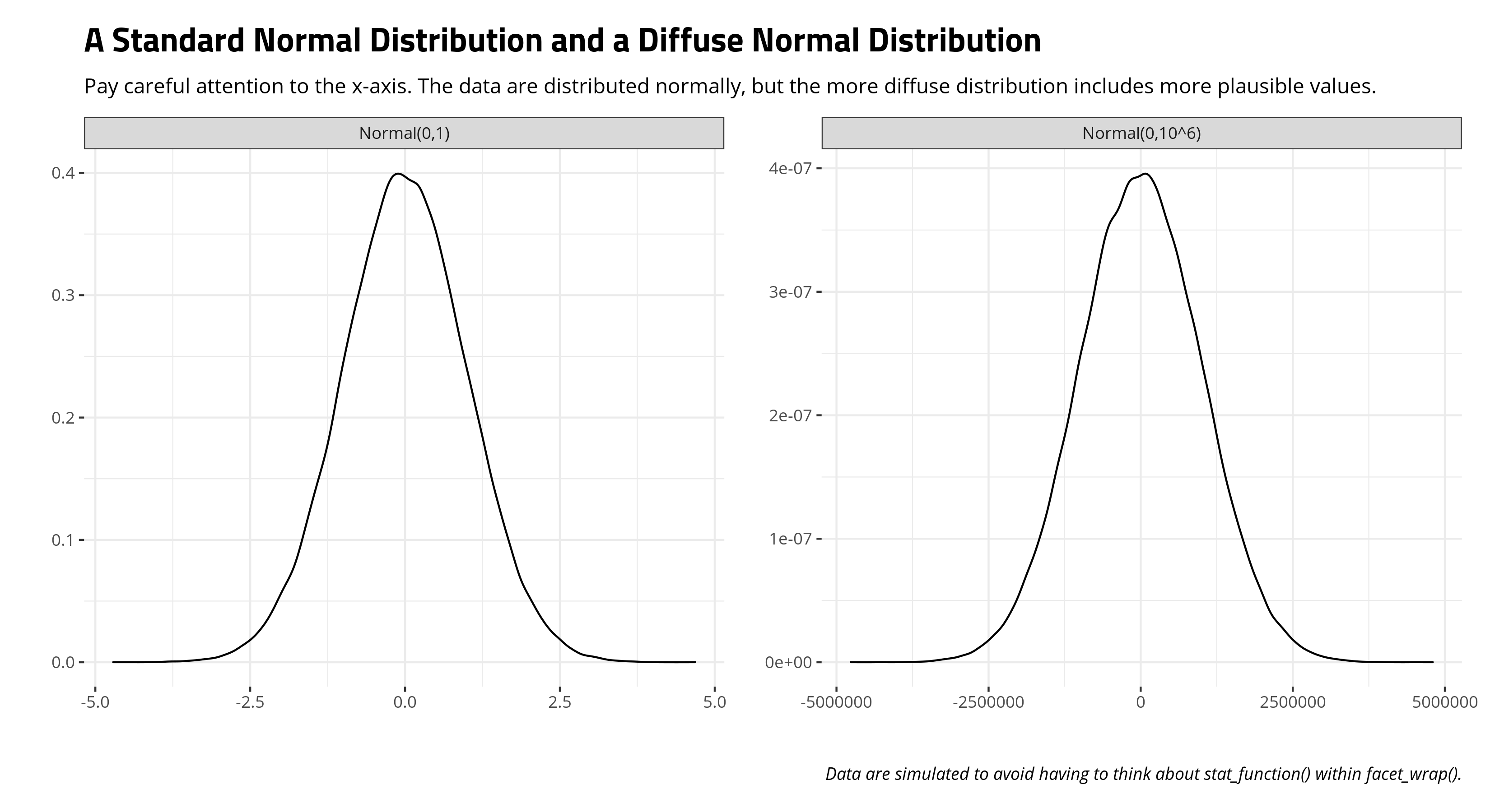
Here’s an illustration of what this means. Because you, the researcher, are electing to not think carefully about your data, {brms} is having to think about it for you in a way that at least gets the prior distribution process out of the way so that it can do its thing. In a case like this, {brms} begins by assuming the following values are at least possible. I’ll balance this out with a consideration of some other common Student’s t distributions in the Bayesian modeling world.
jenny()
tibble(`student_t(3,0,1)` = rstudent_t(100000, 3, 0, 1),
       `student_t(3,0,2.5)` = rstudent_t(100000, 3, 0, 2.5),
       `student_t(3,0,10)` = rstudent_t(100000, 3, 0, 10),
       `student_t(3,0,25.4)` = rstudent_t(100000, 3, 0, 25.4),
       `student_t(3,55.1,25.4)` = rstudent_t(100000, 3, 55.1,25.4),) -> t_examples
Our first introduction to Student’s t-distribution came with a focus on the “standard” t-distribution that was more interested in the degrees of freedom. This three-parameter (aka: “location-scale”) version is a bit more flexible and more diffuse. You should be able to see how long those tails go in this three-parameter version of Student’s t-distribution above. Consider its corollary: the standard normal distribution. You remember that it’s a near impossibility to observe a value more extreme than 3 on either side of the standard normal distribution. However, those extremes are a bit more common with a Student’s t-distribution.
jenny()
t_examples %>%
  select(1:3) %>%
  # for funsies
  mutate(`Normal(0,1)` = rnorm(100000, 0, 1)) %>%
  gather(var, val) %>%
  group_by(var) %>%
  mutate(mean  = mean(val),
         range50 = paste0("[",round(quantile(val, .25), 2),
                          ",",round(quantile(val, .75), 2),"]")) %>%
  filter(val <= -3 | val >= 3) %>%
  group_by(var) %>%
  mutate(min = min(val),
            max = max(val),
            n = n(),
            prop = paste0(round((n/100000)*100, 2), "%")) %>%
  slice(1) %>% select(-val)
| Distribution | Mean | 50% Range | Min. | Max. | Number of Observations More Extreme Than -3 or 3 | % of Extreme Observations |
|---|---|---|---|---|---|---|
| Normal(0,1) | 0.00 | [-0.67,0.67] | -4.71 | 4.68 | 303 | 0.3% |
| student_t(3,0,1) | 0.00 | [-0.77,0.77] | -57.43 | 77.31 | 5643 | 5.64% |
| student_t(3,0,10) | 0.02 | [-7.6,7.64] | -373.10 | 505.81 | 78150 | 78.15% |
| student_t(3,0,2.5) | -0.01 | [-1.92,1.91] | -68.30 | 173.34 | 31674 | 31.67% |
In other words, if you’re not going to think about your data, {brms} will think about it for you, if only a little, just so that it can proceed with the actual stuff you want. It will default to a Student’s t-distribution that will be something it thinks is sensible. However, because it does not know the full details of your data-generating process, it will provide some longer tails to hedge its bets.
Have {rstanarm} Think of Priors For You
You could also elect to have {rstanarm} think of priors for you. Gelman et al. (2020) explain this in some detail in Regression and Other Stories, which is a book you should definitely buy. The approach that Gelman and company describe is a “soft constraint” that is important when data are sparse. More commonly, you’ll see this described as a “weakly informative” approach to priors.
In their application, Gelman and company are leaning on what we know about a standard normal distribution. We all learned about about 99% of the observations in a standard normal distribution is going to be within about 2.58 standard units from the mean. Gelman and company round that to 2.5 to allow a little more wiggle room. However, {rstanarm} cannot assume that the data you have are standardized all the way around (i.e. for both the outcome and your given independent variables) and therefore it’s going to divide the standard deviation of the dependent variable over the standard deviation of a given independent variable and multiply that by 2.5 to get a standard deviation for a normal distribution with a mean of zero. For the y-intercept, it will set a prior distribution to be normal with a mean equal to the mean of the dependent variable with a standard deviation that is 2.5 times the standard deviation of y. Like {brms}, {rstanarm} is peeking at your data to figure out areas in which to start exploring because you elected to not think about your data.
uniondensity %>%
  summarize(sd_y = sd(union),
            mean_y = mean(union),
            sd_y25 = sd_y*2.5,
            sd_left = 2.5*sd_y/sd(left),
            sd_size = 2.5*sd_y/sd(size),
            sd_concen = 2.5*sd_y/sd(concen),
            rate_sigma = 1/sd_y) %>% data.frame
#>       sd_y mean_y   sd_y25  sd_left  sd_size sd_concen rate_sigma
#> 1 18.75283 54.065 46.88208 1.387893 28.85946   145.092 0.05332528
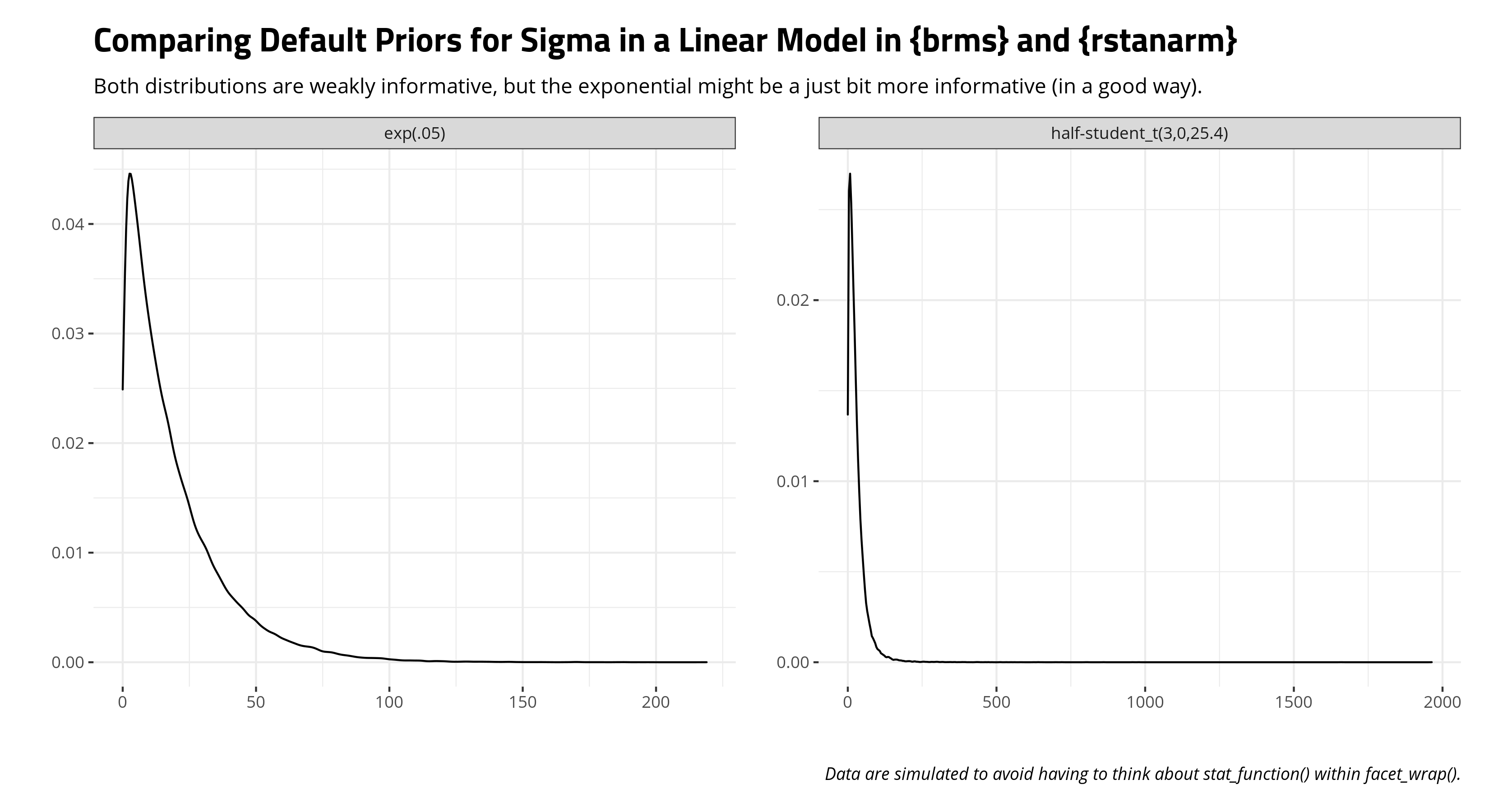
The only major divergence is that {rstanarm} eschews the half-t or half-normal distribution for the residual standard deviation and slaps an exponential distribution with rate equal to 1 over the standard deviation of the dependent variable. Here’s what it would look like compared to a “half”-t that {brms} would employ. Both are weakly informative, but I rather like the {rstanarm} approach here in that 1) it’s explicitly non-negative and 2) slightly more informative than the more diffuse “half”-t that {brms} is using. I’ve yet to see a residual standard deviation of like 2,000. I’m sure it’s out there, but I haven’t seen it in my travels.
Think of Your Own “Reasonable Ignorance” Priors
The final approach here to use your head to make some reasonably informed priors based off what you know or anticipate about the data. I think this is the hardest for beginners to do because it implies subjectivity or deck-stacking. If you do it well, it just means you know at least a little about the data. If you elect to not know a little about your data, you’re punting to software to do it for you. That could lead to prior distributions that really don’t make sense and can only bog down computation.
Using our union density data, we already know a few things about the data. For one, the dependent variable has a theoretical minimum and maximum of 0 and 100. Neither are observed; there is no advanced country in which 1) no one in the entire country is unionized and 2) 100% of the workforce is unionized. No matter, we know that about our data in advance of actually observing it. That’s important prior information by itself and it’s going to have implications for our y-intercept. Had we read about Wilensky’s (1981) measure of left-wing governments, we’d know there were a lot of different values possible that range from 0 (e.g. the United States) to the 100s (i.e. Sweden). Thus, the coefficient for that independent variable is going to have to be small, saying nothing about the discernibility of the coefficient from a counterclaim of zero effect. We might also know that the concentration variable has an effective range of about 0 to a little over two. The size variable has a fairly small range as well in terms of units of 1. If we have prior information in the form of even knowing what a regression coefficient is, and electing (for now), to not standardize our independent variables, we’d know the coefficients for the logged labor force and industrial concentration variables are going to be rather large (again saying nothing for the moment about discernibility from zero).
Thus, here’s an approach to impose what I think of as “reasonable ignorance” priors, given beforehand knowledge of the data (and with only a tiny bit of peeking in a way that I don’t think is going to bother a Bayesian too much). Let’s focus on the left-wing index variable to start and conjure a situation in which that variable—and that variable alone—is 100% the driver of union density. No other variable matters at all. Let’s assume, reasonably, that it’s positive (though it’s immaterial for what happens here). We’re going to assume that 0 and 100 are theoretically possible (if effectively impossible) observations of the dependent variable and that 0 and 120 are conceivable bounds of the left-wing index variable. In the near ludicrous situation in which left-wing governments are 100% the driver of union density, that means the dependent variable would equal 0 when the left-wing government variable is 0. When the left-wing variable is 120, the observation of the dependent variable would be 100 (the theoretical maximum). A potential maximum effect then could be identified when \((100-0) = (120-0)*x\). Solve for x, where \((100-0)/(120-0) = x\), and you get a hypothetical maximum effect of a unit-change in left-wing governments, the absolute value of which is about .83. Two things stand out here: 1) it cannot possibly be more than that in either direction and 2) it’s unlikely to be that because it would be observed in a situation in which it alone was responsible for union density to the exclusion of all other factors. That just isn’t realistic. Thus, we want to treat that as a potential tail in a distribution that stops just about there. Given what we know about a normal distribution, and that about 99% of the distribution is within about 2.58 standard units from the mean, we can divide that potential maximum effect by 2.58 (which comes out to about .32) and treat it as the standard deviation of a normal distribution with a mean of 0. We could try to squeeze that further, but by going with the approximate z-value for a 99% interval rather than the approximate z-value for a 99.9% interval, we allow the prior to “keep the change”, so to say.
We could do the same for the other independent variables. Let’s assume just for sake of illustration that the hypothetical min-max range of the industrial concentration variable is [0, 2.5]. Under a similar ludicrous situation where it was the only driver of union density, the maximum unit effect is 40. Scale that by 2.58 and the prior we’ll stick on the industrial concentration variable is a mean of 0 and a standard deviation of 15.5. The logged labor force size requires some care here. Namely, we know it can’t be 0. Indeed, there is no 0. The minimum is 4.39 (Iceland), which is unsurprising. The maximum is 11.4 (the United States). If we round that to a conceivable minimum of 4 and a maximum of 12 (i.e. they don’t get much smaller than Iceland or bigger than the U.S. among the population we’re describing), we’ll get a maximum unit effect of 12.5. Scale that by 2.58 and we’ll assign a prior distribution with a mean of 0 and standard deviation of 4.84.
All that remains are priors for the y-intercept and the residual standard deviation of the model. There’s going to be one problem with the prior for the y-intercept. Namely, 0 cannot possibly occur for the labor force size variable. Indeed, the hypothetical minimum is 4. If you had potential or actual 0s for the other variables, I’d recommend a similar prior here that might, say, start at 50 and not really reach below 0 or above 100. However, your y-intercept is already going to be uninformative and, worse yet, you’re not going to immediately know in which way unless you build in prior beliefs about the direction of these effects (which I’m electing to not do). That said, 0 occurs for the other two variables, so I know those are going to pull a y-intercept to between 0 and 100. However, the logged labor force size variable could well push the y-intercept to be outside 0 or 100. I might be able to get away with this by sticking a y-intercept prior to have a mean of 50 and a standard deviation of 25. I think it’s going to be within the scale, but I’ll have to be diffuse and use this as a cautionary tale to scale your data. Here, I’ll borrow the {rstanarm} approach to putting a prior on the residual standard deviation from the exponential distribution. Now that I’ve read that, I’m going to do that by default for my Bayesian linear models.
This creates priors that look like this.
reasonable_priors <- c(set_prior("normal(0,.32)", class = "b", coef= "left"),
                         set_prior("normal(0,4.84)", class = "b", coef="size"),
                         set_prior("normal(0,15.5)", class="b", coef="concen"),
                         set_prior("normal(50, 25)", class="Intercept"),
                         set_prior("exponential(.05)", class="sigma"))
Compare these reasonable ignorance priors with the more diffuse priors that {brms} or {rstanarm} are providing for you because you’re asking software to think of your data instead of thinking about it yourself. You’re bringing prior information into this analysis. In other words, you know what values are impossible. For the values that are possible, you at least know they’re highly unlikely. That’s a reasonable approach (I think) to ignorance priors. It’s not deck-stacking. It’s just knowing what you’re doing and knowing what’s possible.
What Different Priors Can Do to Our Inferences
Here are the effects of these various priors can have on our inferences about union density, beyond what Western and Jackman (1994) did in their article and what I reproduced here. Again, this is a fair bit of code so I’ll only show the finished result.
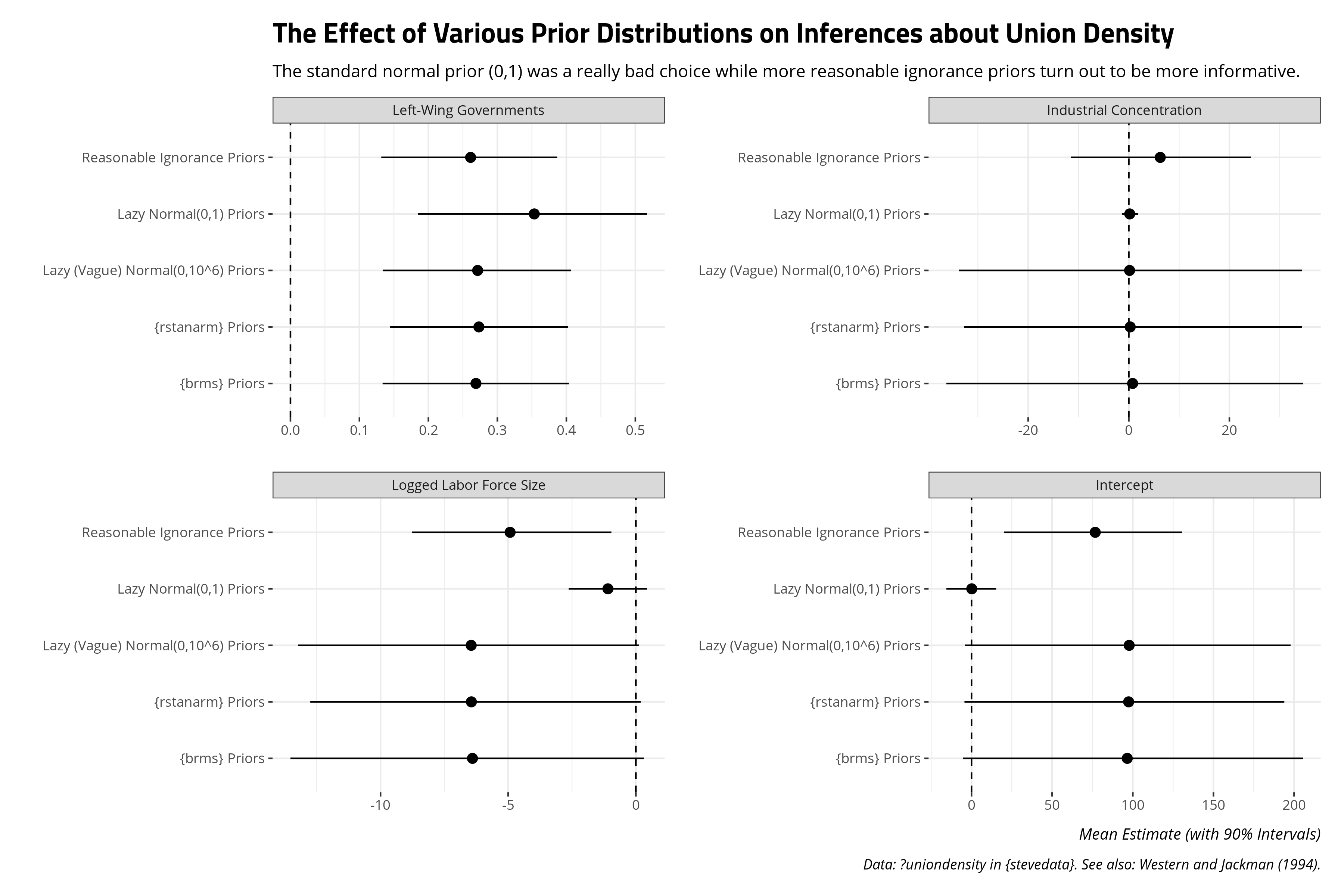
The results of these different priors point to a few things worth discussing. First, one thing that immediately stands out to me is the lazy standard normal prior, with a mean of 0 and a standard deviation of 1, was kind of an idiot prior. It was an idiot prior for a lot of reasons. For one, I attached it to the intercept, which was stupid. I had no earthly reason to believe that intercept would functionally be between -3 and 3. I got lucky with the left-wing government coefficient, in that the true effect of left-wing governments was always going to be in those smaller bounds. However, there was good reason to expect that the two other variables would have plausible effects outside the basic bounds of a standard normal distribution. I elected to be an idiot with that prior information by slapping on a standard normal distribution on those effects. There are plenty of applications in which a standard normal distribution is a good, honest ignorance prior for a model. This was not one of them. This was an idiot prior, an illustration of what being an idiot with prior distributions can do to inferences.
The more diffuse priors that come default in {brms} and {rstan} produce results that look broadly similar to the lazy normal “vague” prior with a mean of 0 and a standard deviation of a million. The inferences that come from it suggest what we know from Western and Jackman (1994). Left-wing governments have that expected, positive effect that is discernible from a counter-claim of zero effect. There’s also good reason to believe that Wallerstein is correct and Stephens is wrong. Logged labor force size has a mostly discernible, negative effect on union density while industrial concentration has an effect that is practically zero effect.
However, I want to draw attention to the reasonable ignorance priors because I think the results communicate something that is 1) more interesting from a substantive standpoint and 2) more informative for students. Recall we have just 20 observations and 16 degrees of freedom. It’s a low-power analysis so our prior expectations of the data are going to exert a fairly strong influence on the posterior distribution of results. With that in mind, and knowing what we know about the data, why on earth are we choosing to believe that a one-unit change in a given independent variable could change the dependent variable by something like a million? We know that’s impossible. The dependent variable has a theoretical minimum and maximum. It can’t be less than 0 and it can’t be more than 100. However, those incredibly diffuse priors are leaving open a possibility that is just not possible.
Use your head here too. We identified that the potential maximum effect of something like logged labor force size on union density, one way or the other, would be a case where a one-unit change in logged labor force size increases/decreases union density by about 12.5 percentage points. That’s the maximum effect. The moment we don’t see something like that is the moment we can start ruling that out. However, the weak nature of the data and some incredibly diffuse priors suggest that it’s still possible when we can probably start ruling it out. That’s in part why those bounds on logged labor force size are so diffuse. With weak data and diffuse priors that are lazily thinking about your data (because you are electing to not think about your data), the posterior distribution of results comes with bounds you could probably start dismissing. I think a new statistics students will just see that the whiskers for the reasonable ignorance prior are further removed from 0 than the more diffuse priors, but they will miss the important reason why. Reasonable ignorance is important information. Use it.
To Stephens’ credit too, it suggests something that’s probably a bit more realistic about industrial concentration. Diffuse priors suggest the effect is practically zero effect. It could well be zero, but shouldn’t we have some reason to believe (from the literature) that the effect probably leans more positive than negative? It could still be zero (and thus potentially negative as well). However, such a diffuse result that hovers almost exactly on zero came because we could have thought more about our data and elected to not do so. The end result doesn’t vindicate Stephens’ hypothesis, per se, but it looks more plausible because we thought about our data beyond slapping on a go-go-gadget lazy normal prior or having our software think about our data and priors for us.
Conclusion: How Should You Think About Your Priors?
I’ll defer to people who are smarter than me on how to think about priors, but I’ll close with the following things based on what I think are clever/reasonable for most substantive applications, with an eye toward teaching students about priors. There are certainly more complex models and priors than I can plausibly teach or even know myself (i.e. I’ll confess to knowing nothing about Dirichlet distributions), so my aim here is the family of linear and generalized linear models.
First, I’m still of the mentality that you should always scale your non-binary inputs, preferably by two standard deviations rather than one. Make zero occur or be plausible everywhere so that your y-intercept amounts to an estimated value of y for what’s a typical case. That’ll also aid what prior you put on your y-intercept.
Toward that end, I actually rather like the {rstanarm} approach to calculating prior distributions for the residual standard deviation. I think you can peek “little a” at your data, as a treat. It’s technically cheating for a pure Bayesian, but only the fundamentalist will make an issue of it. I rather like the exponential prior to the half-normal or half-t because the exponential distribution doesn’t cluster at zero. Your residual standard deviation won’t either.
If you scale your non-binary inputs by two standard deviations rather than one, the effect of a one-unit change in an independent variable on a dependent variable is going to be the effect of a change across about 47.7% of the independent variable. That’s quite a magnitude effect. You can use that for thinking of reasonable ignorance priors.
Knowing what you know about logistic regressions and the logistic distribution, I think a standard normal distribution on the regression coefficients does well in most applications. If you think you have a potential separation problem, a normal distribution with a mean of 0 and standard deviation of 2.5 has worked well for me in the past.
For most applications, you may be overthinking the prior by asking things like whether you should go with a Cauchy prior or a normal prior or a Student’s t prior. When in doubt, use functions available in {brms} or—a hidden R package gem—{LaplacesDesmon}—to simulate some data from these distributions to see what they look like. Use those functions to get an idea of what you might be thinking for a prior distribution.
Importantly, though, if you can avoid those default priors in {brms} and {rstanarm}, do it. It’s not the package authors’ fault that those priors are diffuse. They’re there because you’re probably asking them to think of your data for you when you should be thinking of your data instead. My particular applications are often plenty data-rich, albeit with important random effects that I need to model, so I don’t have the weak data problem that I present here. However, those default priors can really bog down computation time. If you’re curious, my experience has suggested that Student’s t (3,0,1) is adequate for the standard deviations of my random effects while a normal distribution with a mean of 0 and a standard deviation of 2.5 works well for the other parameters (in the logistic regression context).
One thing I appreciate about the Bayesian approach is that makes what was old into new again. Decades ago, researchers with little computational power had to think carefully about their model before dropping punch cards off at the mainframe for a weekend. Cheap computing power came with some lazy thinking about the data and the model (and let he who is without sin cast the first stone). The Bayesian approach brings some of that back full circle. The model can take some time, so you should think of ways to do the job right. Think a little about your data. Think a little about your model. It’ll go a long way.
-
But, tl;dr: Bayes is actually giving an answer to the inferential question you’re asking and posterior distributions are more intuitive for quantities of interest. ↩
Disqus is great for comments/feedback but I had no idea it came with these gaudy ads.