Bootstrap Your Standard Errors in R, the Tidy Way

- The Toxicity of Heteroskedasticity
Last updated: 28 April 2021
This will be another post I wish I can go back in time to show myself how to do when I was in graduate school. It’s something I recently taught my grad class how to do as part of a lab session.
Most of my research questions don’t have solutions easily amenable to ordinary least squares (OLS) regression, whether because my main outcomes of interest are non-interval or because I’m freely confessing up front that I have important spatial/temporal heterogeneity that is important to model on its own terms. Still, the quantitative policy studies people love OLS and we all learn it first. However, as I caution, a model is only as useful as the assumptions that underpin it. When the assumptions that underpin it are violated, the model’s output becomes suspect in some ways.
One of those important assumptions of an OLS model that’s easy to violate in a social science application is that of homoskedasticity. The flip side of this, in as many words, is that the variability of our variable is unequal across the range of our variables that we believe explain it. This is “heteroskedasticity.” More formally, the deviation between fitted value and the prediction error depends on an x-value. We often see this manifest in a “cone of shame”, though this is just the most obvious/illustrative way we observe it. The implications for violating this assumption of homoskedasticity mostly concern our standard errors around our coefficients. They may be too large or too small, which could lead to either a Type 1 or Type 2 error.
There are various “solutions” for heteroskedasticity, which are less “solutions” (since it may hinge on the kind of heteroskedasticity and whether you know it or not). In practice, these solutions are more robustness tests to compare with your standard error estimates derived from a simple OLS model. One of those solutions is “bootstrapping”, which was first introduced by Efron (1979) as an extension of the “jackknife” approach. Briefly, the “jackknife” approach first introduced by Quenouille (1949), and given its name by Tukey (1958), is a “leave-one-out” resampling method that recalculates a statistic of interest iteratively until each observation has been removed once. One limitation from this, beyond how tricky it is to adapt to more complex data structures, is jackknifing struggles with smaller data sets and the number of resamples is capped at the number of observations. Bootstrapping, a resampling with replacement approach to calculating statistics of interest (e.g. standard errors from a regression), is far more versatile and flexible.
Bootstrapping, like Bayesian inference, is another thing that mystified me in graduate school since learning it often meant being bombarded with instruction that cared more about notation than implementation. Learning statistics through Stata confounded matters, mostly because a simple call in a regression did the bootstrapping for you without explaining it (i.e. the reverse problem). Here, I’ll hope to make it more transparent and explain what’s happening in bootstrapping standard errors that both shows how to do it and explains what bootstrapping is doing.
First, here are the R packages that I will be using for this exercise, followed by a discussion of the data.
library(tidyverse) # main workflow, which has purrr and forcats (IIRC)
library(stevemisc) # misc. functions of interest to me, Steve
library(stevedata) # my toy data package
library(lmtest) # for a Breusch-Pagan test for heteroskedasticity
# library(broom) # for tidying model output, but not directly loaded
library(knitr) # for tables
library(kableExtra) # for pretty tables
library(modelr) # for bootstrap
library(ggrepel) # one-off use for annotating a fitted-residual plot
The Data and the Problem
The data I’m using are probably familiar to those who learned statistics by Stata. It’s some statewide crime data from around 1993 or so that come available in Agresti and Finlay’s Statistical Methods for the Social Sciences since around its third edition in 1997. I ganked these data from the internet and added it to my {stevedata} package as the af_crime93 data. The data include 51 observations (i.e. 50 states + DC, which should be a state) and you can read more about it here. I used this data set for this application because I know in advance these data are going to flunk a Breusch-Pagan test for heteroskedasticity.
Supposed we wanted to explain the violent crime rate per 100,000 people in the population (violent) as a function of the percentage of the state with income below the poverty level (poverty), the percentage of families in the state headed by a single parent (single), the percent of population in metropolitan areas (metro), the percentage of the state that is white (white), and the percentage of the state that graduated from high school (highschool). The ensuing regression formula—and pretty output with help from the {broom}, {knitr}, and {kableExtra} packages—would look like this. The output suggests all but the white variable and the highschool variable have statistically significant effects. Remember that p-value for the white variable, since it’s hovering around .10. This would be almost statistically significant at a lower threshold that we typically use for smaller data sets.
M1 <- lm(violent ~ poverty + single + metro + white + highschool, af_crime93)
| Term | Coefficient | Standard Error | t-statistic | p-value |
|---|---|---|---|---|
| Intercept | -1795.904 | 668.788 | -2.685 | 0.010 |
| % Poverty | 26.244 | 11.083 | 2.368 | 0.022 |
| % Single Family Home | 109.467 | 20.360 | 5.377 | 0.000 |
| % Living in Metro Areas | 7.609 | 1.295 | 5.874 | 0.000 |
| % White | -4.483 | 2.779 | -1.613 | 0.114 |
| % High School Graduate | 8.646 | 7.826 | 1.105 | 0.275 |
However, people who report OLS models should also provide some diagnostic tests to explore whether the assumptions of the model hold. One of those assumptions is homoskedasticity, which can be tested with a Breusch-Pagan test from the {lmtest} package. Here, the test output is testing a null hypothesis of homoskedastic variances. If the p-value is low enough to your particular threshold—we’ll go with p < .05—you should reject the null hypothesis of homoskedastic variance and assert you instead have heteroskedastic variances in your model. The output of the Breusch-Pagan test suggests we’ve violated the assumption of homoskedasticity with these data.
broom::tidy(bptest(M1)) %>%
  kable(., format="html", table.attr='id="stevetable"',
        col.names=c("BP Statistic", "p-value", "Degrees of Freedom", "Method"),
        caption = "A Breusch-Pagan Test for Heteroskedasticity in our Model",
        align=c("c","c","c","l"))
| BP Statistic | p-value | Degrees of Freedom | Method |
|---|---|---|---|
| 15.3974 | 0.0087926 | 5 | studentized Breusch-Pagan test |
A fitted-residual plot will also suggest we don’t have neat-looking variances either.
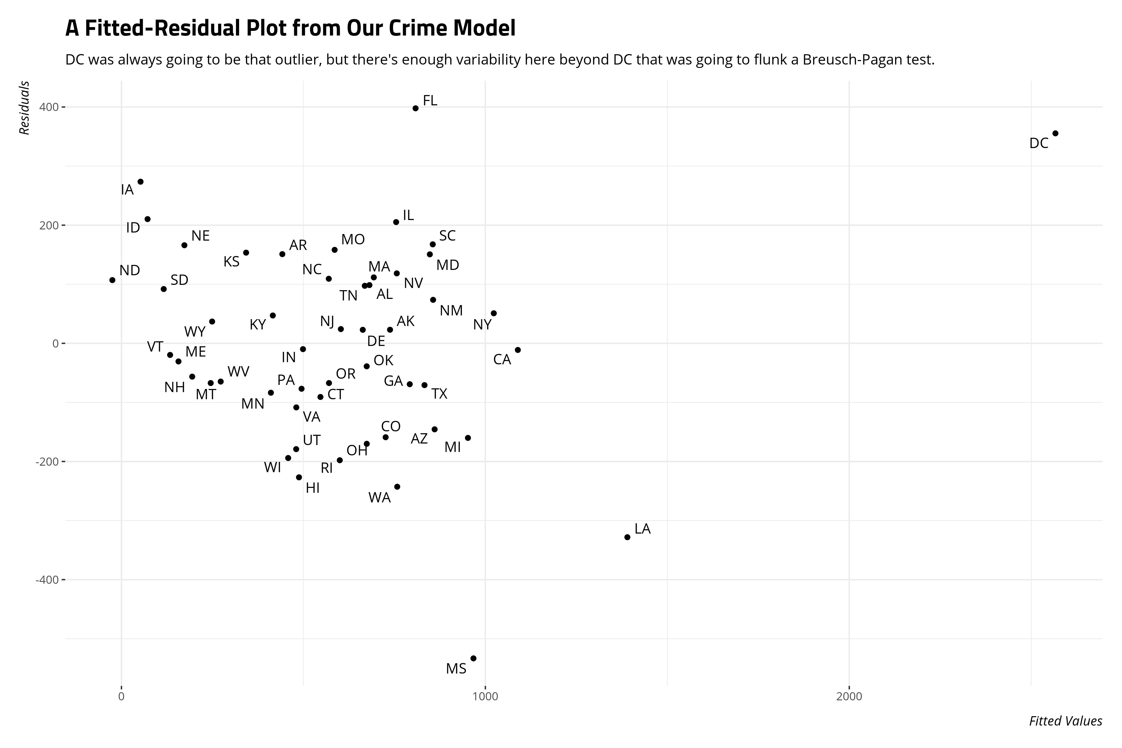
The implication of this kind of heteroskedasticity is less about our coefficients and more about the standard errors around them. Under these conditions, it makes sense to bootstrap the standard errors to compare them to what the OLS model produces.
Bootstrapping, the Tidy Way
{modelr} and {purrr} will make bootstrapping a cinch. Recall that a bootstrap approach is a resampling method, with replacement, that can be done as many times as you want. Since the af_crime93 dataset is rather small and the model is simple, let’s go for a 1,000 bootstrap resamples with {modelr}. Let’s also set a reproducible seed so anyone following along will get identical results. Do note that {modelr} has a separate bootstrap() function that will conflict with a different bootstrap() function in {broom}. I want the {modelr} version and situations like this is why I tend to never directly load {broom} in my workflow.
set.seed(8675309) # Jenny, I got your number...

af_crime93 %>%
  bootstrap(1000) -> bootCrime
The bootstrap() function from {modelr} created a special tibble that contains 1,000 resamples (with replacement, importantly) of our original data. This means some observations in a given resample will appear more than once. You can peek inside these as well. For example, let’s look at the first resample and arrange it by state to see how some states appear more than once, and some don’t appear at all. Notice some observations appear multiple times. Illinois appears three times in these 51 rows; Colorado is even in there five times! Some states, like Alaska and Wyoming, don’t appear at all. That’s fine because there’s no doubt Alaska and Wyoming will be represented well across the 999 other resamples we’re doing and that not every resample is going to have Colorado in it five times.
bootCrime %>%
  slice(1) %>% # grab the first row in this special tbl
  pull(strap) %>% # focus on the resample, momentarily a full list
  as.data.frame() %>% # cough up the full data
  arrange(state) %>% # arrange by state, for ease of reading
  select(-murder) %>% # this is another DV you could use, but not in this analysis.
  # let's pretty it up now
   kable(., format="html", table.attr='id="stevetable"',
        col.names=c("State", "Violent Crime Rate", "% Poverty", "% Single Family Home",
                    "% Living in Metro Areas", "% White", "% High School Graduate"),
        caption = "The First of Our 1,000 Resamples",
        align=c("l","c","c","c","c","c","c","c"))
| State | Violent Crime Rate | % Poverty | % Single Family Home | % Living in Metro Areas | % White | % High School Graduate |
|---|---|---|---|---|---|---|
| AL | 780 | 17.4 | 11.5 | 67.4 | 73.5 | 66.9 |
| AR | 593 | 20.0 | 10.7 | 44.7 | 82.9 | 66.3 |
| CA | 1078 | 18.2 | 12.5 | 96.7 | 79.3 | 76.2 |
| CO | 567 | 9.9 | 12.1 | 81.8 | 92.5 | 84.4 |
| CO | 567 | 9.9 | 12.1 | 81.8 | 92.5 | 84.4 |
| CO | 567 | 9.9 | 12.1 | 81.8 | 92.5 | 84.4 |
| CO | 567 | 9.9 | 12.1 | 81.8 | 92.5 | 84.4 |
| CO | 567 | 9.9 | 12.1 | 81.8 | 92.5 | 84.4 |
| CT | 456 | 8.5 | 10.1 | 95.7 | 89.0 | 79.2 |
| DE | 686 | 10.2 | 11.4 | 82.7 | 79.4 | 77.5 |
| FL | 1206 | 17.8 | 10.6 | 93.0 | 83.5 | 74.4 |
| FL | 1206 | 17.8 | 10.6 | 93.0 | 83.5 | 74.4 |
| GA | 723 | 13.5 | 13.0 | 67.7 | 70.8 | 70.9 |
| HI | 261 | 8.0 | 9.1 | 74.7 | 40.9 | 80.1 |
| HI | 261 | 8.0 | 9.1 | 74.7 | 40.9 | 80.1 |
| IA | 326 | 10.3 | 9.0 | 43.8 | 96.6 | 80.1 |
| ID | 282 | 13.1 | 9.5 | 30.0 | 96.7 | 79.7 |
| ID | 282 | 13.1 | 9.5 | 30.0 | 96.7 | 79.7 |
| IL | 960 | 13.6 | 11.5 | 84.0 | 81.0 | 76.2 |
| IL | 960 | 13.6 | 11.5 | 84.0 | 81.0 | 76.2 |
| IL | 960 | 13.6 | 11.5 | 84.0 | 81.0 | 76.2 |
| IN | 489 | 12.2 | 10.8 | 71.6 | 90.6 | 75.6 |
| KS | 496 | 13.1 | 9.9 | 54.6 | 90.9 | 81.3 |
| KY | 463 | 20.4 | 10.6 | 48.5 | 91.8 | 64.6 |
| LA | 1062 | 26.4 | 14.9 | 75.0 | 66.7 | 68.3 |
| MA | 805 | 10.7 | 10.9 | 96.2 | 91.1 | 80.0 |
| MA | 805 | 10.7 | 10.9 | 96.2 | 91.1 | 80.0 |
| MD | 998 | 9.7 | 12.0 | 92.8 | 68.9 | 78.4 |
| MD | 998 | 9.7 | 12.0 | 92.8 | 68.9 | 78.4 |
| ME | 126 | 10.7 | 10.6 | 35.7 | 98.5 | 78.8 |
| MN | 327 | 11.6 | 9.9 | 69.3 | 94.0 | 82.4 |
| MO | 744 | 16.1 | 10.9 | 68.3 | 87.6 | 73.9 |
| NC | 679 | 14.4 | 11.1 | 66.3 | 75.2 | 70.0 |
| NC | 679 | 14.4 | 11.1 | 66.3 | 75.2 | 70.0 |
| ND | 82 | 11.2 | 8.4 | 41.6 | 94.2 | 76.7 |
| NJ | 627 | 10.9 | 9.6 | 100.0 | 80.8 | 76.7 |
| NY | 1074 | 16.4 | 12.7 | 91.7 | 77.2 | 74.8 |
| OH | 504 | 13.0 | 11.4 | 81.3 | 87.5 | 75.7 |
| OK | 635 | 19.9 | 11.1 | 60.1 | 82.5 | 74.6 |
| OR | 503 | 11.8 | 11.3 | 70.0 | 93.2 | 81.5 |
| PA | 418 | 13.2 | 9.6 | 84.8 | 88.7 | 74.7 |
| PA | 418 | 13.2 | 9.6 | 84.8 | 88.7 | 74.7 |
| SD | 208 | 14.2 | 9.4 | 32.6 | 90.2 | 77.1 |
| TX | 762 | 17.4 | 11.8 | 83.9 | 85.1 | 72.1 |
| TX | 762 | 17.4 | 11.8 | 83.9 | 85.1 | 72.1 |
| VA | 372 | 9.7 | 10.3 | 77.5 | 77.1 | 75.2 |
| VT | 114 | 10.0 | 11.0 | 27.0 | 98.4 | 80.8 |
| VT | 114 | 10.0 | 11.0 | 27.0 | 98.4 | 80.8 |
| WI | 264 | 12.6 | 10.4 | 68.1 | 92.1 | 78.6 |
| WI | 264 | 12.6 | 10.4 | 68.1 | 92.1 | 78.6 |
| WV | 208 | 22.2 | 9.4 | 41.8 | 96.3 | 66.0 |
Now, here’s where the magic happens that will show how awesome {purrr} is for these things if you take some time to learn it. For each of these 1,000 resamples, we’re going to run the same regression from above and store the results in our special tibble as a column named lm. Next, we’re going to create another column (tidy) that tidies up those linear models. Yes, that’s actually a thousand linear regressions we’re running and saving a tibble. Tibbles are awesome.
bootCrime %>%
    mutate(lm = map(strap, ~lm(violent ~ poverty + single + metro + white + highschool,
                     data = .)),
           tidy = map(lm, broom::tidy)) -> bootCrime
If you were to call the bootCrime object at this stage into the R console, you’re going to get a tibble that looks kind of complex and daunting. It is, by the way, but we’re going to make some sense of it going forward.
bootCrime
#> # A tibble: 1,000 × 4
#>    strap               .id   lm     tidy
#>    <list>              <chr> <list> <list>
#>  1 <resample [51 x 8]> 0001  <lm>   <tibble [6 × 5]>
#>  2 <resample [51 x 8]> 0002  <lm>   <tibble [6 × 5]>
#>  3 <resample [51 x 8]> 0003  <lm>   <tibble [6 × 5]>
#>  4 <resample [51 x 8]> 0004  <lm>   <tibble [6 × 5]>
#>  5 <resample [51 x 8]> 0005  <lm>   <tibble [6 × 5]>
#>  6 <resample [51 x 8]> 0006  <lm>   <tibble [6 × 5]>
#>  7 <resample [51 x 8]> 0007  <lm>   <tibble [6 × 5]>
#>  8 <resample [51 x 8]> 0008  <lm>   <tibble [6 × 5]>
#>  9 <resample [51 x 8]> 0009  <lm>   <tibble [6 × 5]>
#> 10 <resample [51 x 8]> 0010  <lm>   <tibble [6 × 5]>
#> # … with 990 more rows
If you were curious, you could look at a particular OLS result with the following code. You’re wanting to glance inside a list inside a tibble, so the indexing you do should consider that. I’m electing to not spit out the results in this post, but this code will do it.
# here's the first linear regression result
bootCrime$tidy[[1]]

# here's the 1000th one
bootCrime$tidy[[1000]]
Now, this is where you’re going to start summarizing the results from your thousand regressions. Next, we should pull the tidy lists from the bootCrime tibble and “map” over them into a new tibble. This is where the investment into learning {purrr} starts to pay off. It would be quite time-consuming to do this in some other way.
bootCrime %>%
  pull(tidy) %>%
  map2_df(., # map to return a data frame
          seq(1, 1000), # make sure to get this seq right. We did this 1000 times.
          ~mutate(.x, resample = .y)) -> tidybootCrime
If you’re curious, this basically just ganked all the “tidied” output of our 1,000 regressions and binded them as rows to each other, with helpful indices in the resample column. Observe:
tidybootCrime
#> # A tibble: 6,000 × 6
#>    term        estimate std.error statistic      p.value resample
#>    <chr>          <dbl>     <dbl>     <dbl>        <dbl>    <int>
#>  1 (Intercept) -1150.      660.      -1.74  0.0886              1
#>  2 poverty        28.7      10.5      2.75  0.00861             1
#>  3 single         71.1      22.3      3.19  0.00260             1
#>  4 metro           8.61      1.28     6.73  0.0000000258        1
#>  5 white          -1.72      2.15    -0.803 0.426               1
#>  6 highschool      1.46      8.11     0.179 0.858               1
#>  7 (Intercept) -1175.      845.      -1.39  0.171               2
#>  8 poverty        51.0      12.6      4.06  0.000193            2
#>  9 single         11.9      28.5      0.418 0.678               2
#> 10 metro           7.92      1.28     6.21  0.000000154         2
#> # … with 5,990 more rows
This next code will calculate the standard errors. Importantly, bootstrap standard errors are the standard deviation of the coefficient estimate for each of the parameters in the model. That part may not be obvious. It’s not the mean of standard errors for the estimate; it’s the standard deviation of the coefficient estimate itself.
tidybootCrime %>%
  # group by term, naturally
  group_by(term) %>%
  # This is the actual bootstrapped standard error you want
  summarize(bse = sd(estimate)) -> bseM1
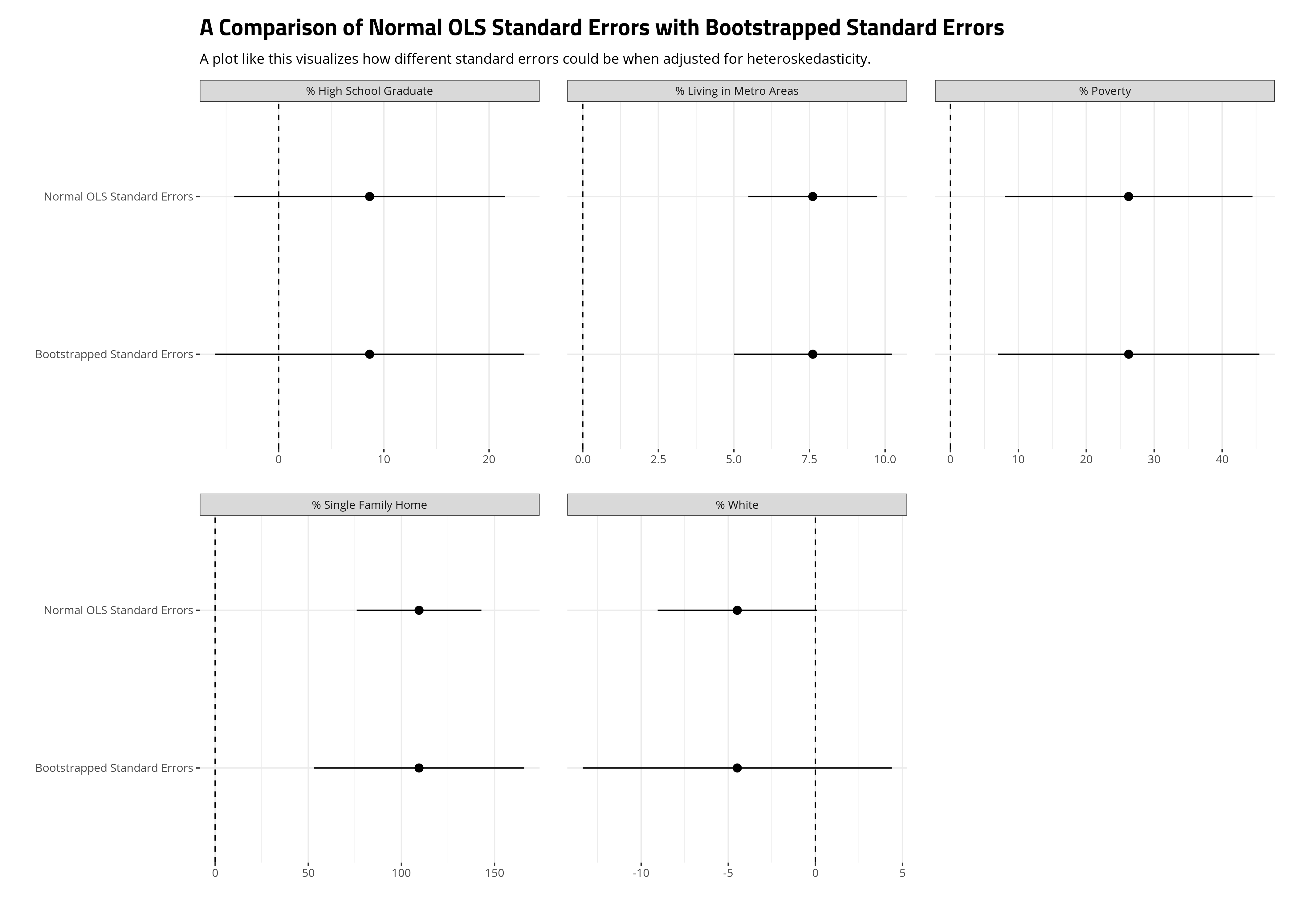
When you bootstrap your standard errors under these conditions, you should compare the results of these bootstrapped standard errors with the standard OLS standard errors for the parameters in your model. Here, we’ll do it visually. The ensuing plot suggests the standard errors most influenced by the heteroskedasticity in our model are those for the single family home variable and especially the percentage of the state that is white variable. In the former case, the bootstrapping still produced standard errors that could rule out a counterclaim of zero relationship, but the percentage of the state that is white variable becomes much more diffuse when its standard errors are bootstrapped. Sure, the 90% confidence intervals that we’re using here (given the small number of observations) would still slightly overlap zero with the OLS estimates, but it was close. It’s not close when the standard errors are bootstrapped. We should be cautious about wanting to make an argument for a precise effect there in our model.
broom::tidy(M1) %>%
  mutate(category = "Normal OLS Standard Errors") %>%
  # This will be convoluted, but I know what I'm doing.
  # Trust me; I'm a doctor.
  bind_rows(., broom::tidy(M1) %>% select(-std.error) %>% left_join(., bseM1 %>% rename(std.error = bse))) %>%
  mutate(category = ifelse(is.na(category), "Bootstrapped Standard Errors", category),
         tstat = estimate/std.error,
         pval = 1.645*pt(-abs(tstat),df=45), # dfs from M1
         lwr = estimate - 1.645*std.error,
         upr = estimate + 1.645*std.error) %>%
  filter(term != "(Intercept)") %>% # ignore the intercept
  mutate(term = forcats::fct_recode(term,
                                    "% Poverty" = "poverty",
                                    "% Single Family Home" = "single",
                                    "% Living in Metro Areas" = "metro",
                                    "% White" = "white",
                                    "% High School Graduate" = "highschool")) %>%
   ggplot(.,aes(category, estimate, ymin=lwr, ymax=upr)) +
  theme_steve_web() +
  geom_pointrange(position = position_dodge(width = 1)) +
  facet_wrap(~term, scales="free_x") +
  geom_hline(yintercept = 0, linetype="dashed") +
  coord_flip() +
  labs(x = "", y="",
       title = "A Comparison of Normal OLS Standard Errors with Bootstrapped Standard Errors",
       subtitle = "A plot like this visualizes how different standard errors could be when adjusted for heteroskedasticity.")
Conclusion
Once you understand what bootstrapping is, and appreciate how easy it is to do with {modelr} and some {purrr} magic, you might better appreciate its flexibility. If you have a small enough data set with a simple enough OLS model—which admittedly seems like a relic of another time in political science—bootstrapping with this approach offers lots of opportunities. One intriguing application here is bootstrapping predictions from these 1,000 regressions. In other words, we could hold all but the poverty variable constant, set the poverty variable at a standard deviation above and below its mean, and get predictions across those 1,000 regressions and summarize them accordingly.
Either way, bootstrapping is a lot easier/straightforward than some texts let on. If it’s not too computationally demanding (i.e. your data set is small and doesn’t present other issues of spatial or temporal clustering), you could do lots of cool things with bootstrapping. The hope is this guide made it easier.
Disqus is great for comments/feedback but I had no idea it came with these gaudy ads.