Visualizing Random Measurement Error in R
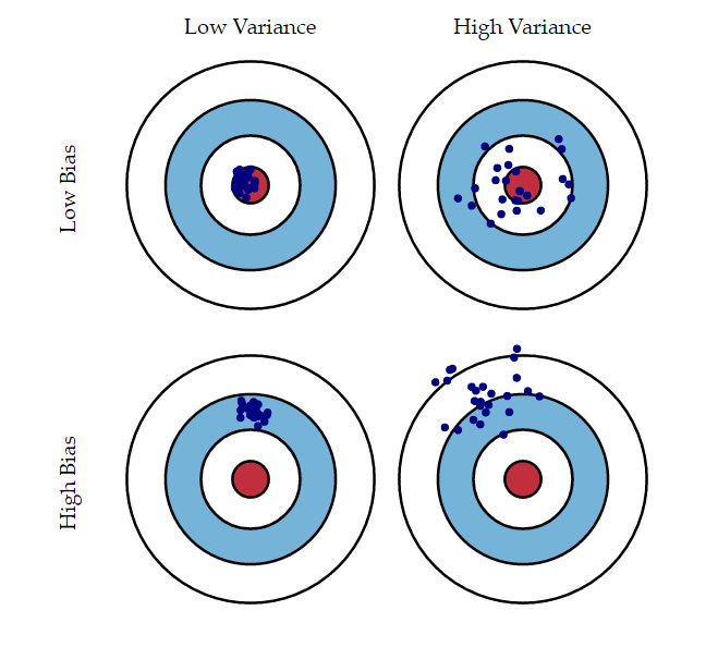
- I think we all get the bullseyes as metaphors of measurement error when we get taught this stuff in graduate school.
Introduction
I’m preparing a week’s lecture/discussion section and lab on measurement error in my graduate-level methods class. The thought occurred to put some of what I intend to do in that class here on my website so, next time I see it, I could think of ways to improve it in the next iteration of the class in another semester. New preps are always a pain and a first class is a guinea pig of a kind.
Briefly: students learning quantitative methods must consider two forms of measurement error. The first is random (stochastic) measurement error. These are deviations in the recorded value that is neither a function of the “true” signal being measured nor deviations that emerge in predictable and constant ways. Systematic measurement error is when the recorded values differ from the “true” values to be measured in a way that is both consistent and predictable. Students learn that neither is necessarily ideal but that systematic measurement error is a bigger concern than random measurement error. For one, random measurement error is built into a lot of what applied statisticians do. Indeed, random assignment purposesly introduces random error into our design the extent to which treatment and control groups could differ, if randomly, beyond the systematic introduction of a treatment. Second, systematic measurement error has the unwelcome effect of pulling our measurements off their “true” value in the population. Thus, systematic measurement error creates mismeasures of the “concept” or “signal” in question. The bullseyes illustrate this and most textbooks use them as a metaphor for the two concepts.
This understanding of systematic and random measurement error will touch on related things students learn. Again, briefly, systematic measurement error coincides with measurement “bias.” In the measurement sense, “bias” means the measure includes something else beyond just what the measurement purports to capture. My go-to for a social science audience is the problem of measuring “political tolerance” during the Cold War by reference to whether Americans would allow communists or atheists to run for elected office or give a speech in the respondent’s town. The measure that follows, by assuming “least-liked groups” of communists and atheists, measured political tolerance. It also measured political ideology, religiosity, and variable fear of the Soviet Union that gradually waned from the peak of the mid-1950s through the mid-1970s. The “political tolerance” example is nice jumping-off point to what “bias” implies for inferences. Bias means our measures are “invalid” and our inferences are likely to be “biased” as well.
Random measurement error creates some problems as well, though we don’t treat these as the same scale of danger as we do the problems typically associated with systematic measurement error. Generally, random measurement error coincides with “unreliable” estimates that have a higher “variance.” The noise in our estimates often eliminates the possibility of making inferences. We call this a “Type 2 error.” In other words, a true relationship exists but we are unable to proverbially detect the signal from the din we measured. To be fair, this is unwelcome and we should not be content with it. But, we tell students (and learned ourselves) that it is worse to misrepresent a relationship that does not objectively exist than it is to fail to detect a relationship that actually does exist.
Anywho, here’s some R code to think about teaching this stuff, with a focus at least on random measurement error. Yes, I know I ramble.
R Code
Here are some R packages you’ll need for this post. Check the _rmd directory for my website on Github for the full thing since I may likely condense some of the code because graphs, for example, are code-heavy.
library(tidyverse)
library(stevemisc)
library(stargazer)
I recently added a cor2data() function to my {stevemisc} package. It will take any correlation matrix and simulate data from it that is just rnorm(n, 0, 1) for all variables named in the matrix. The underlying code is effectively identical to what I did here to introduce potential readers/students to instrumental variable analysis.
In this case, we’ll create a data set of 1,000 observations with the following correlation matrix. There are just an x1, an x2, and an error term e. Nothing is correlated in any meaningful way. From this correlation matrix, we’ll create 1,000 observations with my go-to reproducible seed. Thereafter, we’re going to create an outcome y that is a simple linear function of all three things. In other words, x1 and x2 objectively change y by 1 with each unit increase in x1 or x2 (plus or minus some random error e) and the estimated value of y when x1 and x2 are zero is 1.
vars = c("x1", "x2",  "e")
Cor <- matrix(cbind(1, 0.001, 0.001,
                    0.001, 1, 0.001,
                    0.001, 0.001, 1),nrow=3)
rownames(Cor) <- colnames(Cor) <- vars

# from {stevemisc}
Data <- cor2data(Cor, 1000, 8675309) # Jenny I got your number...

Data$y <- with(Data, 1 + 1*x1 + 1*x2 + e)
Here is a simple OLS model regressing y on x1 and x2 (along with some other regressions looking at just x1 and x2). The coefficients that emerge from the OLS model are in orbit what the true population effects are. However, it is worth noting the effect of x1 is more than two standard errors from the true population effect. The difference is not huge or necessarily immediately noticeable, but it’s worth mentioning.
| Dependent variable: | |||
| y (Outcome) | |||
| Just x1 | Just x2 | Full Model | |
| (1) | (2) | (3) | |
| x1 | 0.909*** | 0.913*** | |
| (0.046) | (0.033) | ||
| x2 | 0.983*** | 0.986*** | |
| (0.044) | (0.033) | ||
| Constant | 0.985*** | 0.978*** | 0.981*** |
| (0.046) | (0.044) | (0.033) | |
| Observations | 1,000 | 1,000 | 1,000 |
| Adjusted R2 | 0.283 | 0.336 | 0.622 |
| Note: | *p<0.1; **p<0.05; ***p<0.01 | ||
Random Measurement Error in X
We can show what random measurement error does to our inferences with these parameters in mind and through this setup. When I talk to undergraduates about random measurement error in the coding sense, I talk about having, say, a lazy undergraduate working for me coding fatalities in a conflict. However, this hypothetical coder is lazy and sloppy. In some cases, the coder entered an 11 instead of 1, or a 1000 instead of 100 (or vice-versa). The nature of the coding error is not systematic. It’s just sloppy or lazy. Alternatively: “random.”
Here’s a way of showing this in our setup. For every 10th value in x2 in our data set of 1,000 observations, we will substitute that particular value for some other value that will range from the implausible to the plausible and back again. Since all variables in the data frame are generated randomly from a normal distribution with a mean of zero and a standard deviation of one, this type of coding error is not targeting any subset of the distribution. It does not hinge on whether the 10th value is large or small, positive or negative. The 10th value generated from rnorm() does not depend on the previous value. This is ultimately a way of mimicking random measurement error.
The values we’ll substitute will range from -500 to 500 at various increments. Since x2 is simulated to have a mean of zero and a standard deviation of one, the values we’ll substitute will range from the statistically impossible, given the distribution of the data (e.g. -500), to the plausible (e.g. 0, the mean).
new_vals <- c(-500, -100, -10, -5, -3, -2, -1, 0,
              1, 2, 3, 5, 10, 100, 500)

new_vals <- c(seq(1:4), seq(5, 50, 5), 75, seq(100, 500, 100))

new_vals <- c(new_vals*-1, 0, new_vals)

Xmods <- tibble()


for (i in new_vals) {
# Looping through new_vals
# For every 10th value for x2, recode it to whatever the ith value is in new_vals
Data %>%
  mutate_at(vars("x2"), list(x2nv = ~ifelse(row_number() %in% c(seq(0, 1000, by =10)), i, x2))) -> Data
  # regress y  on this particular new x2nv variable
  mod <- lm(y ~ x1 + x2nv, data=Data)
  # grab r-square
  r2 = broom::glance(mod)[1,1] %>% pull()
  # create a broom table that codes whatever the ith value of new_vals is, and the adjr2 as well
  broomed = broom::tidy(mod) %>% mutate(mod = i, r2 = r2)
  # bind it to Xmods
  Xmods = bind_rows(Xmods, broomed)

}

# grab/broom up M3, for context
M3df <- broom::tidy(M3) %>%
  mutate(lwr = estimate - abs(qnorm(.025))*std.error,
         upr = estimate + abs(qnorm(.025))*std.error)  %>%
  mutate(r2 = broom::glance(M3) %>% pull(1))
Here is way of visualizing what random measurement error in x2 does to inferences we want to make about the relationship between x2 and y. Recall that y is objectively, in part, a function of x2 wherein each unit increase in x2 coincides with an increase of 1 in y even as there is an estimated (and independent) effect of x1 and an error term as well. This amounts to a Type 2 error. The true population effect is 1. Our OLS estimates for x2 without random measurement error includes 1. However, random measurement error pushes the estimated effect to zero and precludes us from detecting that signal. You can call this a “bias” of a sort; random measurement error in an independent variable biases a regression coefficient to zero. I don’t know if we necessarily think of this in the same way we think of “bias” in the systematic context, but that’s because a lot of us were molded in the context of null hypothesis testing.
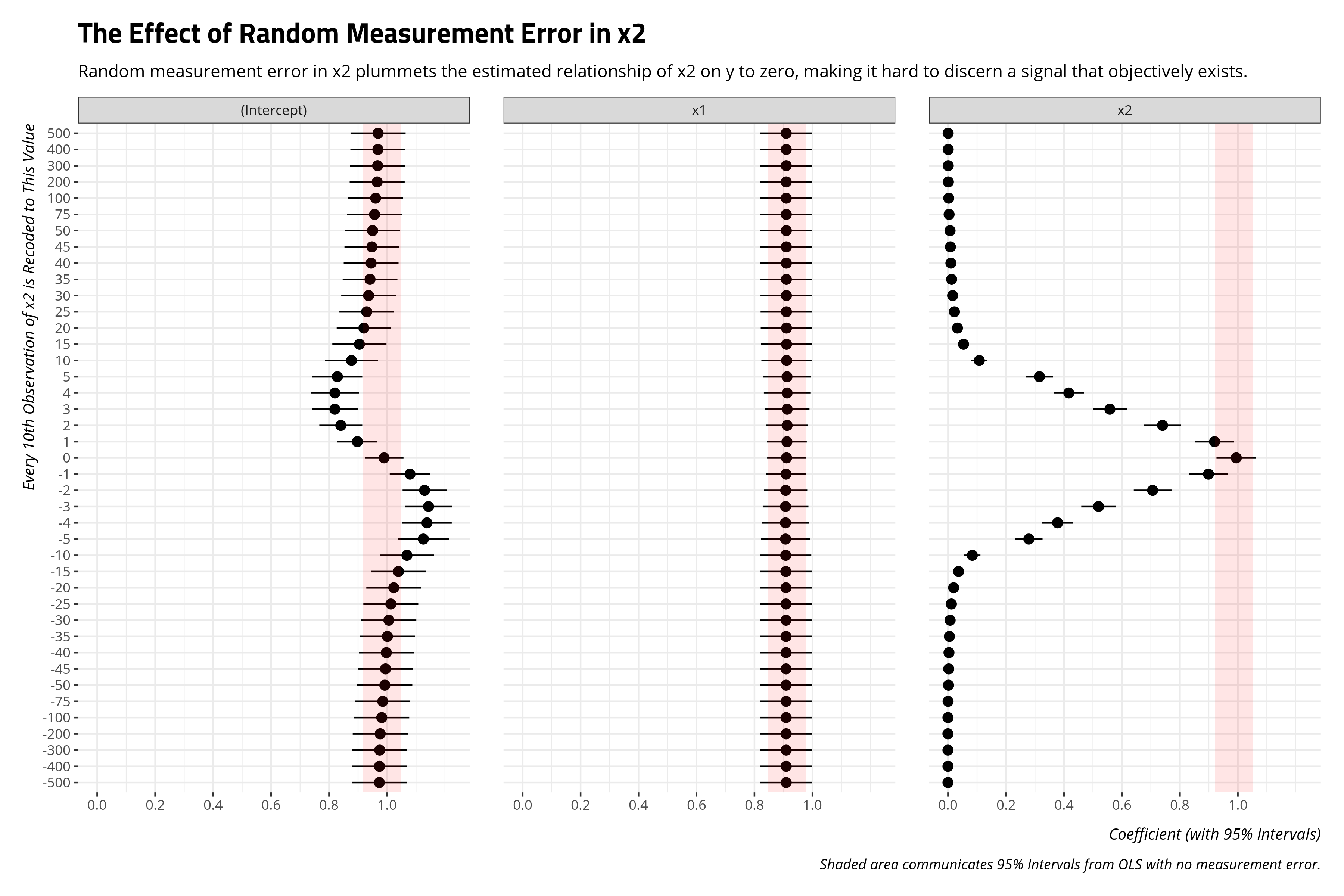
There is an interesting effect on the intercept too. The more, for lack of better term, “plausible” the random measurement error is in the scale of x2 (e.g. recoding every 10th value to be 0, i.e. the mean), the more the intercept is stressed from its true value as well. The less plausible the random measurement error is, the more the intercept is unchanged.
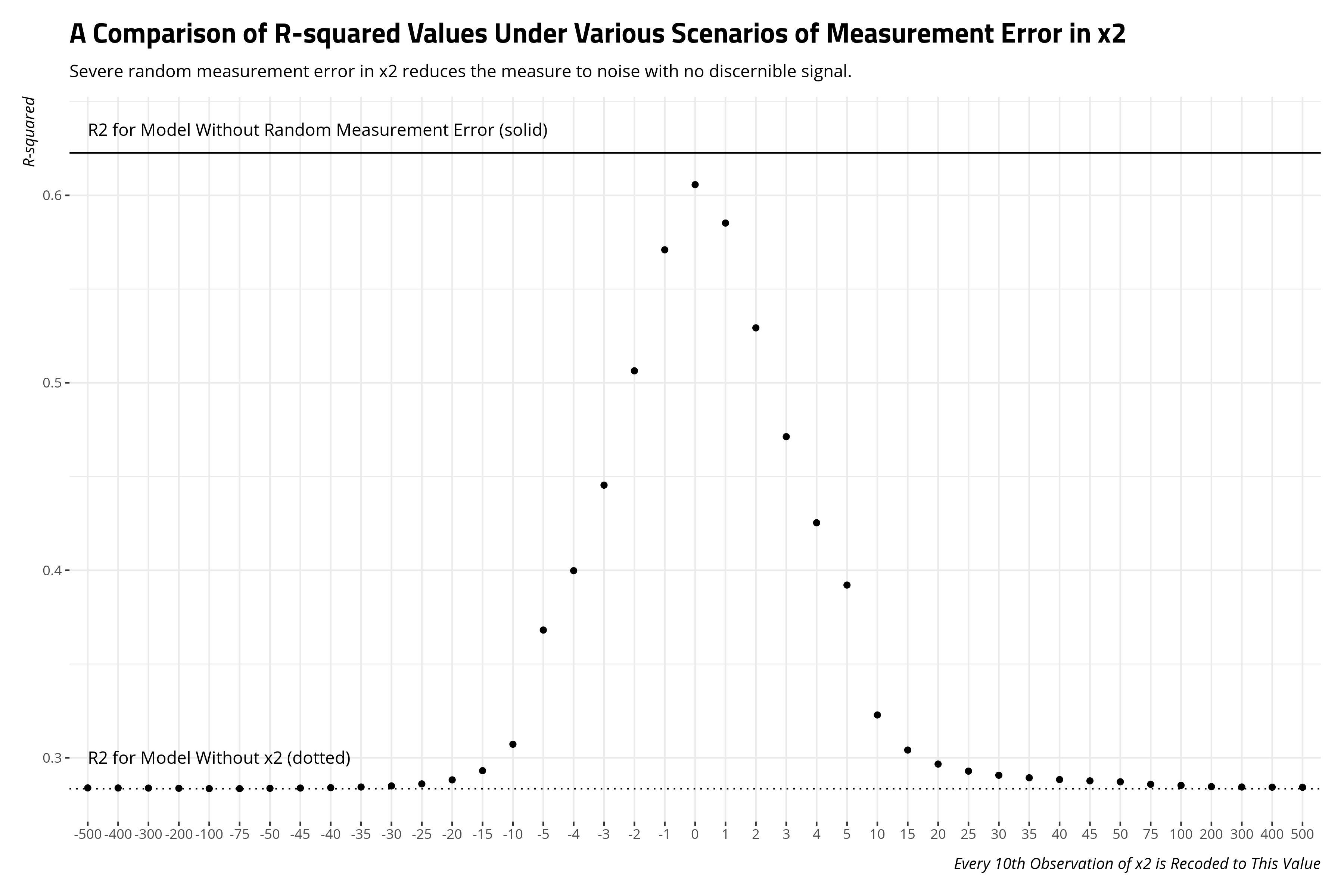
Another way of looking at the fundamental takeaway here is to compare the R-squared values from these models. The effect of increasing measurement error in x2, at least in how I’ve done that in this exercise, is to collapse the R-squared from the model with no measurement bias to the model that excludes x2 outright. Random measurement as severe at both tails reduces the measure of x2 to noise.
Random Measurement Error in Y
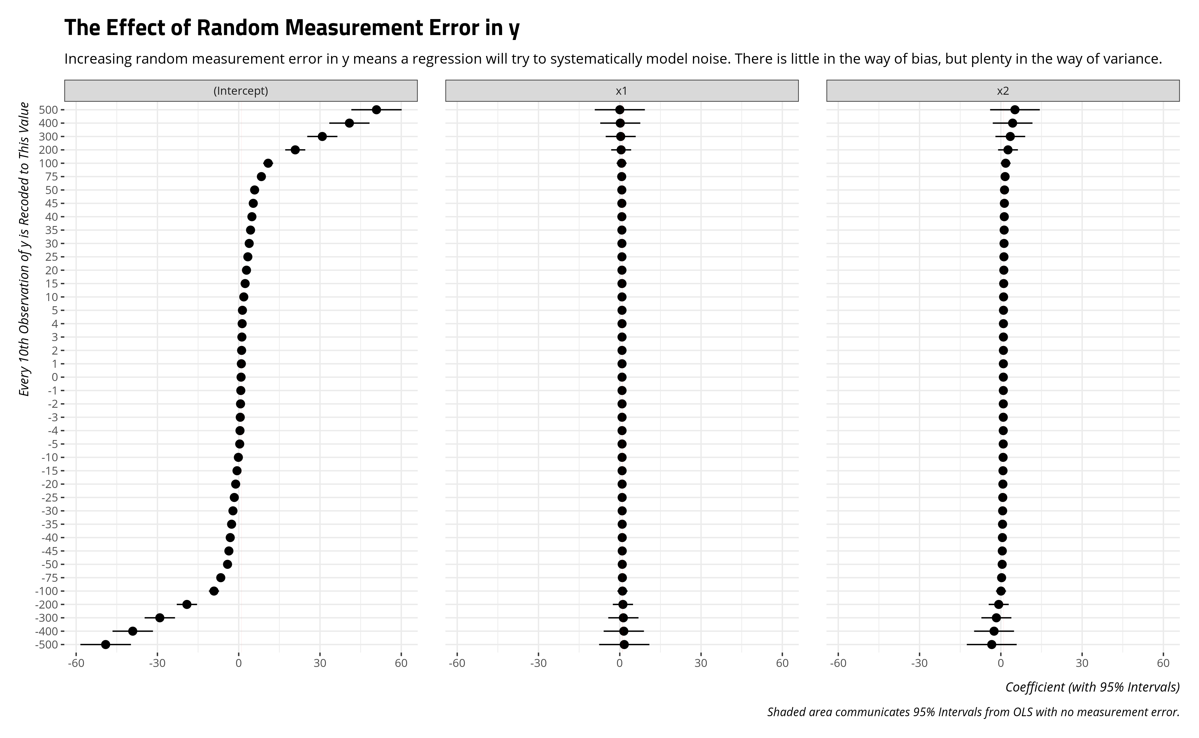
Random measurement error in the dependent variable does not have quite the same effect, even if the fundamental takeaway in terms of what random measurement error does will be the same. We’ll do what we did previously for x2, but for y instead.
Ymods <- tibble()

for (i in new_vals) {
Data %>%
  mutate_at(vars("y"), list(ynv = ~ifelse(row_number() %in% c(seq(0, 1000, by =10)), i, y))) -> Data
  mod <- lm(ynv ~ x1 + x2, data=Data)
  r2 = broom::glance(mod)[1,1] %>% pull()
  broomed = broom::tidy(mod) %>% mutate(mod = i, r2 = r2)
  Ymods = bind_rows(Ymods, broomed)

}
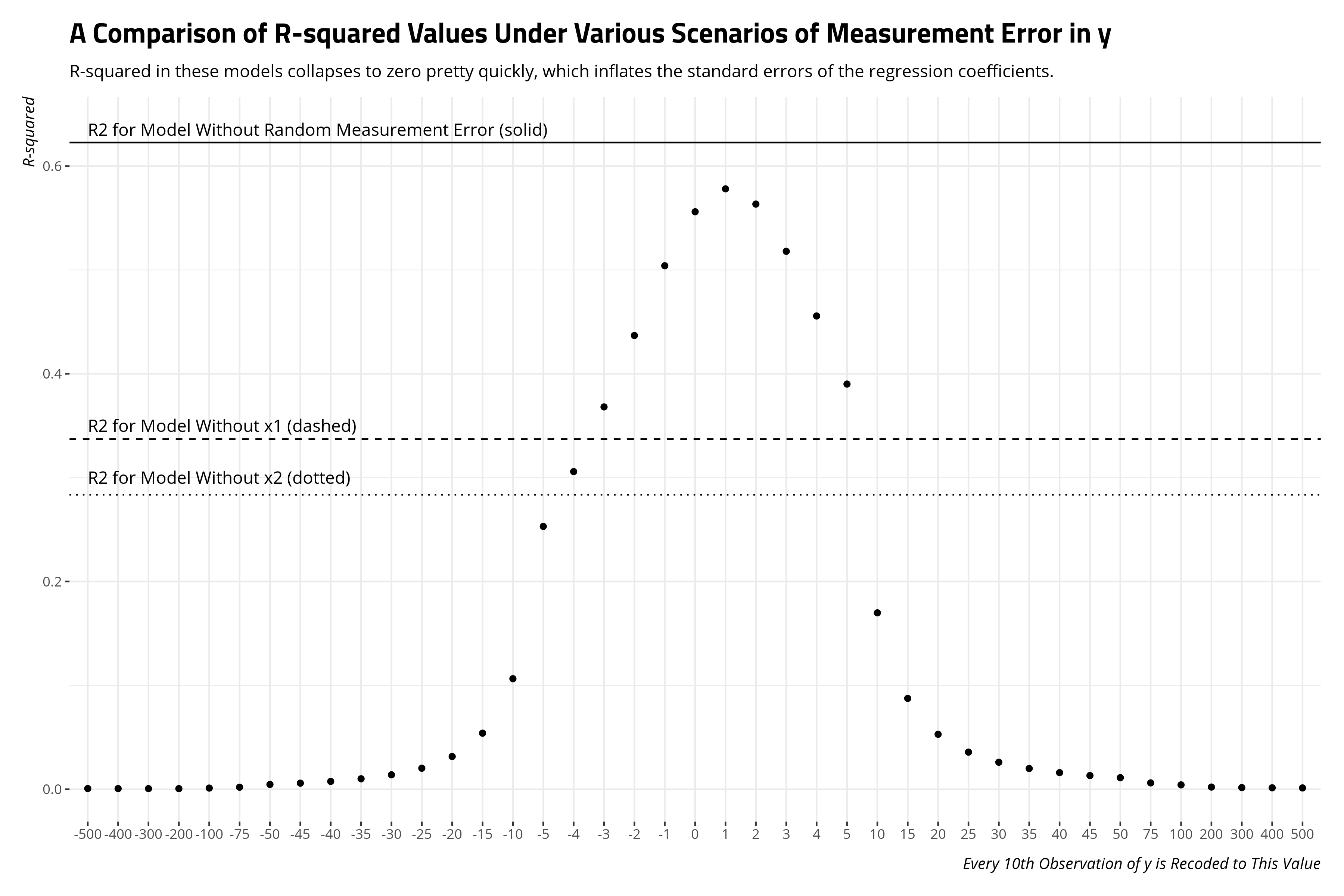
Random measurement error in the dependent variable will not really bias the regression coefficients. The intercept will want to travel in the direction of the random measurement error in y, which isn’t too surprising when you internalize that the intercept is the estimate of y when all covariates are set to zero. However, the regression coefficients for x1 and x2 don’t materially move much. They just get noisier. Random measurement error in an independent variable will push its coefficient to zero. Random measurement error in the dependent variable will extend out the standard errors for the independent variables.
Comparing the R-squared values will illustrate what’s happening here. Random measurement error, whether in an independent variable or a dependent variable, decreases R-squared. The model does not fit the data well because the data are noise.
I should think soon about extending this framework to explore systematic measurement error and bias in this setup. Already, my post on instrumental variables does this. However, I wanted something on my website that at least unpacks random measurement error as well.
Disqus is great for comments/feedback but I had no idea it came with these gaudy ads.