Graphing the Manufacturing Trends Under the Trump Presidency, in R
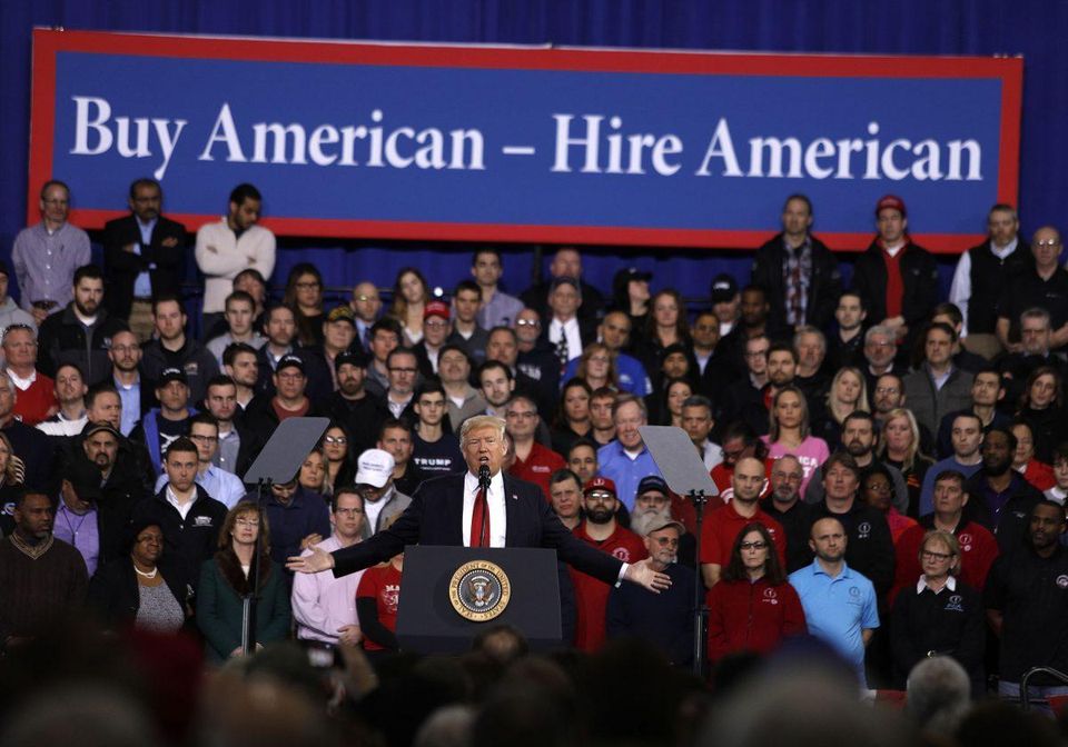
- Global supply chains in 21st century manufacturing are complex if you're smart, but easy if you're an idiot. (Bill Pugliano/Getty Images)
Introduction
Stories like these from Bloomberg and The Washington Post have become near monthly articles in the Trump presidency. The tl;dr, as I tell my students in my introduction to international relations class, is that Trump’s mercantilist worldview is an anachronism in the modern world and with the modern economy operating as it does. Tweeting tariff policy by fiat to “protect” American jobs with the idea of repatriating outsourced jobs home to the United States (and the Rust Belt especially) is a simplistic approach that does more harm than good. With my apologies to Scott Lincicome, tariffs—then and now—fail to achieve their ideal policy aims and just foster economic chaos and political dysfunction along the way. There’s a t-shirt for it and everything.
The explanations for this are multiple, and I’ll try to summarize them here briefly. For one, job outsourcing to areas where labor is cheaper is just one part of the puzzle. You cannot stop firms from maximizing profit and labor is routinely the biggest expense of operating a business. You can physically bar a company from outsourcing jobs to Mexico or China, but you cannot disincentivize a firm from trying to cut labor costs. This is the automation problem. A job that can be automated, will be automated. This is happening everywhere, whether it’s robotic arms in manufacturing automobiles or, well, the automated teller machine in banking. This is going to collide with the declining labor share of income phenomenon that is being observed everywhere. Since it’s easier to switch from labor to capital these days, the relative price of investment goes down and less income accrues to labor as a result. There’s an irony here, though: manufacturing jobs pay more now than they did previously (see slide 28). However, there’s lower demand for lower-skill manufacturing jobs. Those wages are accruing to higher-skill labor, for which there’s more demand.
The idea behind a naive tariff policy like the one Trump has imposed is to repatriate work and output to the United States. Tariffs impose a cost for a firm wanting to buy a foreign product or a product made of a domestic firm from foreign labor, ideally (and simplistically) disincentivizing them from purchasing it relative to a domestic firm’s domestically made product. Curtailing supply while holding demand constant obviously increases price, which could possibly be profit to be shared with the general public or trickled down to labor. If firms are unable to outsource their labor or consume foreign products, and simplistically/wrongly assuming there’s still human work to be done that cannot be automated, then jobs shift from foreign labor to domestic labor for the production of manufacturing outputs. Hire American. Buy American. There’s some underpants gnomes magic working here, leaving aside that American farms (one of our most prominent export-oriented sectors of the economy) are the front line for the inevitable response from a country like China.
The problems here are multiple, again underscoring that a mercantilist worldview is rooted in a myopic centuries-since-discreted economic approach that no longer squares with the nature of the modern economy. Part of the problem that these news reports are getting is these tariffs may be artificially prop, say, steel-producing or aluminum-producing firms but they wreck firms that use these as primary inputs for manufacturing something else. It’s not just “consumers” that “consume” the object of these tariffs. They’re not achieving their primary policy aims. They’re fostering economic dysfunction along the way, certainly in key states, without which, Trump cannot secure re-election in 2020.
You can illustrate what’s happening here with some R code. The source code for this post is available on the _source directory for my website, on Github.
R Code
Here are some R packages you’ll need for this post.
library(fredr)
library(tidyverse)
library(stevemisc)
Next, use the built-in state.abb vector in base R to create two objects that will help us loop through FRED. I’m fairly sure you’ll want an API key for this. Mine is stored in my home R directory. We’ll create a states data frame later for clarity in merging.
# Manufacting employment
statemfgnabbs <- paste0(c(state.abb),"MFGN")
# Total non-farm employment data
statetotempabbs <- paste0(c(state.abb),"NAN")

data.frame(stateabb = state.abb, statename = state.name) -> states
Now, we’ll create two empty tibbles, called Mfgn and Nan, that we’re going to amend with manufacturing employment and total employment data. I know I shouldn’t be doing loops at this stage in my life, but I don’t know of a smarter/sexier way of doing this and it doesn’t take too much time for this to run. Feel free to drop a comment if you know of a smarter/sexier/”tidier” way of doing this.
Mfgn <- tibble()
Nan <- tibble()

for (i in 1:length(statemfgnabbs)) {
  fredr(series_id = statemfgnabbs[i],
        observation_start = as.Date("2017-01-01")) -> hold_this
    bind_rows(Mfgn, hold_this) -> Mfgn
}

for (i in 1:length(statetotempabbs)) {
  fredr(series_id = statetotempabbs[i],
        observation_start = as.Date("2017-01-01")) -> hold_this
    bind_rows(Nan, hold_this) -> Nan
}
Next, we’re going to do some cleaning. I’ll annotate what I’m doing in the code below. Of importance: manufacturing is a yearly cycle in a lot of states. California is illustrative here. Evaluating manufacturing policies at the state-level should be done with 12-month lags.
Mfgn %>%
  # rename value to mfgn. "value" is default fredr output
  rename(mfgn = value) %>%
  # scrape stateabb from the series_id.
  # This works well when you know how series_ids are structured
  mutate(stateabb = stringr::str_sub(series_id, 1, 2)) %>%
  # Left join the unemployment data in, but make sure stateabb aligns
  # get rid of series_id too.
  left_join(., Nan %>%
              mutate(stateabb = stringr::str_sub(series_id, 1, 2)) %>%
              select(-series_id)) %>%
  # rename value (which came from Nan) to be totempnf
  rename(totempnf = value) %>%
  # Create variable for how much manufacturing is a part of state employment
  mutate(percmfgn = (mfgn/totempnf)*100) %>%
  # left_join with the states data frame, which will have actual state names.
  left_join(., states) %>%
  # reorder the columns
  select(date, stateabb, statename, series_id, everything()) %>%
  # group_by state name
  group_by(statename) %>%
  # calculate mean of how much manufacturing employment matters to state employment
  # Then rank it
  mutate(meanpcmfgn = mean(percmfgn)) %>%
  # Thenk rank it
  ungroup() %>%
  mutate(rank = dense_rank(desc(meanpcmfgn))) %>%
  # group by again...
  group_by(statename) %>%
  #  create 12-month difference, a percentage difference
  # And also a variable for if the 12-month difference was negative or not.
  mutate(diff = mfgn - lag(mfgn, 12),
         percdiff = (diff/lag(mfgn, 12))*100,
         neg = ifelse(diff < 0, "Negative", "Positive")) -> Mfgn
We can look across manufacturing employment across all 50 states to see where the most growth and contraction has happened after considering the yearly-cyclical nature of the data. I hide the code for formatting the table but it’s visible in the _source directory. The results show troubling years that seem to cluster in the Midwest, the extent to which the Midwest is home to more manufacturing jobs as a percentage of overall employment. Indiana and Wisconsin saw a contraction of manufacturing jobs in 2019 after controlling for the cyclical nature of manufacturing employment. Even places that were on the balance positive—like Ohio, Michigan, and Illinois—still saw a slowdown in 2019 relative to 2018.
Mfgn %>%
  mutate(year = lubridate::year(date)) %>%
  group_by(statename, year, rank) %>%
  na.omit %>%
  summarize(meandiff = mean(percdiff),
            meandiff = paste0(round(meandiff, 2),"%")) %>%
  ungroup() %>%
  spread(year, meandiff) %>%
  arrange(rank)
| State | Rank | 2018 | 2019 |
|---|---|---|---|
| Indiana | 1 | 1.99% | -0.19% |
| Wisconsin | 2 | 1.75% | -0.37% |
| Michigan | 3 | 2.23% | 0.11% |
| Iowa | 4 | 3.22% | 2.45% |
| Kentucky | 5 | 0.66% | 1.32% |
| Alabama | 6 | 1.35% | 1.29% |
| Arkansas | 7 | 2% | 1.84% |
| Mississippi | 8 | 0.48% | 1.3% |
| Ohio | 9 | 1.72% | 0.52% |
| Kansas | 10 | 2.23% | 1.38% |
| South Carolina | 11 | 2.86% | 3.08% |
| Tennessee | 12 | 1.29% | 1.83% |
| Minnesota | 13 | 0.96% | -0.26% |
| North Carolina | 14 | 1.22% | -0.27% |
| Oregon | 15 | 2.57% | 3.35% |
| New Hampshire | 16 | 2.12% | -0.82% |
| South Dakota | 17 | 3.1% | 3.55% |
| Nebraska | 18 | 1.49% | 0.19% |
| Illinois | 19 | 2.14% | 0.68% |
| Vermont | 20 | 0.9% | 1.86% |
| Connecticut | 21 | 0.99% | 0.58% |
| Pennsylvania | 22 | 1.17% | -0.81% |
| Missouri | 23 | 2.26% | 1.54% |
| Idaho | 24 | 2.8% | 3.03% |
| Georgia | 25 | 1.93% | 0.72% |
| Utah | 26 | 2.95% | 3.78% |
| Washington | 27 | 1.32% | 3.34% |
| Maine | 28 | 1.72% | 2.41% |
| Oklahoma | 29 | 2.92% | -1.37% |
| Rhode Island | 30 | -0.24% | -2.54% |
| California | 31 | 1.07% | 0.95% |
| Texas | 32 | 3.31% | 3.12% |
| Louisiana | 33 | 0.14% | 2.01% |
| Massachusetts | 34 | 0% | -0.49% |
| West Virginia | 35 | 0.87% | 1.38% |
| Virginia | 36 | 2.21% | 2.63% |
| Arizona | 37 | 3.7% | 4.37% |
| New Jersey | 38 | 1.14% | 1.49% |
| North Dakota | 39 | 4.69% | 1.5% |
| Delaware | 40 | 3.02% | 1.66% |
| Colorado | 41 | 2.27% | 1.21% |
| New York | 42 | -0.49% | -0.49% |
| Florida | 43 | 2.36% | 2.65% |
| Montana | 44 | 2.97% | -0.89% |
| Maryland | 45 | 1.26% | 0.03% |
| Nevada | 46 | 15.73% | 8.49% |
| Alaska | 47 | -6.09% | 3.38% |
| Wyoming | 48 | 3.98% | 4.69% |
| New Mexico | 49 | 2.22% | 1.38% |
| Hawaii | 50 | -1.36% | -1.85% |
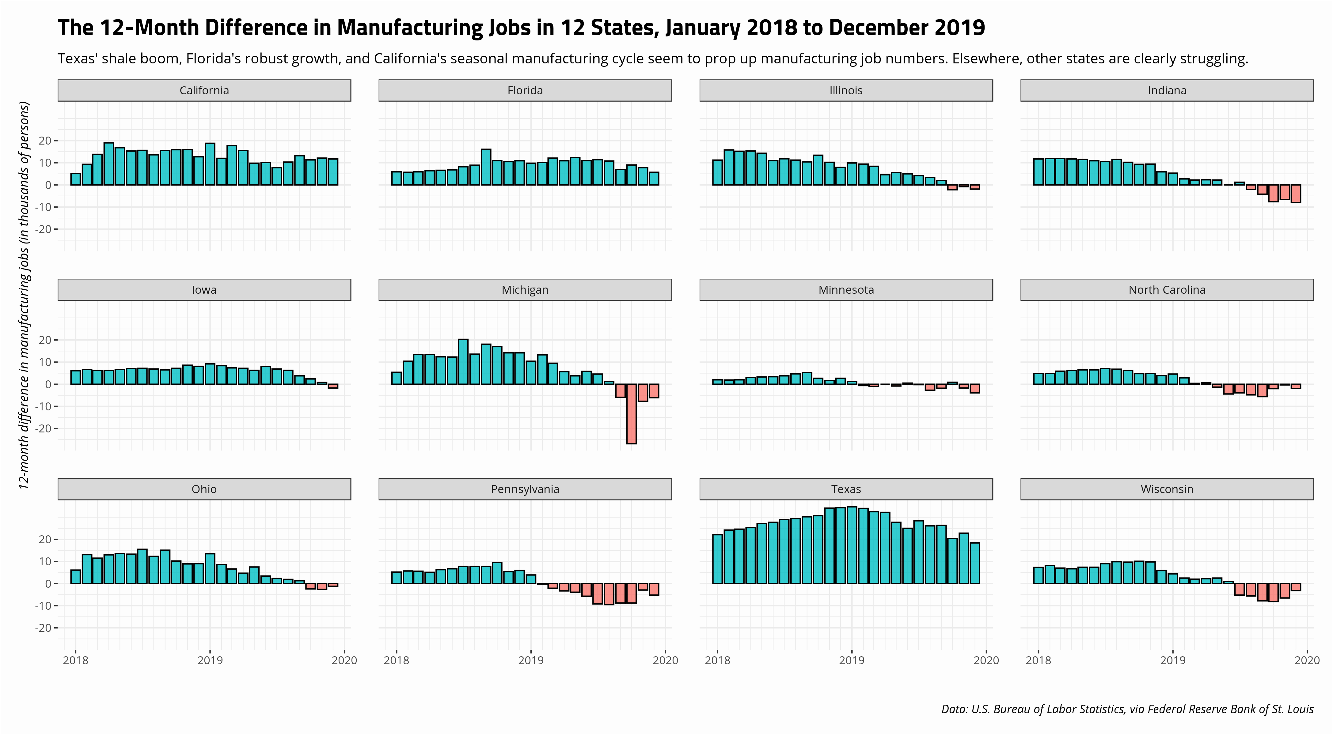
Yearly summaries don’t quite communicate some of what these news reports are saying. In other words, the trends are emerging and more recent months will show that. This graph will communicate how I recommend interpreting the manufacturing employment data in these 12 states of interest. Namely, Texas’ shale boom, Florida’s robust growth, and California’s seasonal manufacturing cycle seem to prop up manufacturing job numbers. There are a lot of states that look like they’re struggling. These are incidentally key states for Trump’s voting bloc. That’s not to say these numbers are sufficient to crack Trump’s support base. Indeed, the basic problem is Trump voters in these areas are being compensated with another form of utility not implied by theories of pocketbook voting.
Nevertheless, what you see here underscores what these news reports are relaying, and how three of our biggest state economies paper over more worrying trends in some states of bigger political interest.
Mfgn %>%
  filter(stateabb %in% c("IA","IL","IN","OH","MI","WI","PA","MN","NC", "FL","CA", "TX")) %>%
  ggplot(.,aes(date, diff, fill = neg)) +
  geom_bar(stat="identity", alpha=0.8, color="black") +
  facet_wrap(~statename) +
  theme_steve_web() + post_bg() +
  scale_x_date(date_breaks = "1 year", date_minor_breaks = "1 month", date_labels = "%Y") +
  labs(title = "The 12-Month Difference in Manufacturing Jobs in 12 States, January 2018 to December 2019",
       x = "",
       caption = "Data: U.S. Bureau of Labor Statistics, via Federal Reserve Bank of St. Louis",
       y = "12-month difference in manufacturing jobs (in thousands of persons)",
       subtitle = "Texas' shale boom, Florida's robust growth, and California's seasonal manufacturing cycle seem to prop up manufacturing job numbers. Elsewhere, other states are clearly struggling.") +
  theme(legend.position = "none")
Disqus is great for comments/feedback but I had no idea it came with these gaudy ads.