What Explains Union Density? A Replication of an Old Article with the {brms} Package
Last updated: 23 June 2021. The data are now in {stevedata} as the uniondensity data frame. You can download this from CRAN. tidy() in {broom} no longer handles {brms} models in the absence of random effects. This post has been updated to reflect those changes. Seeds have been added to the models for reproducibility as well. Some code has been suppressed for presentation.
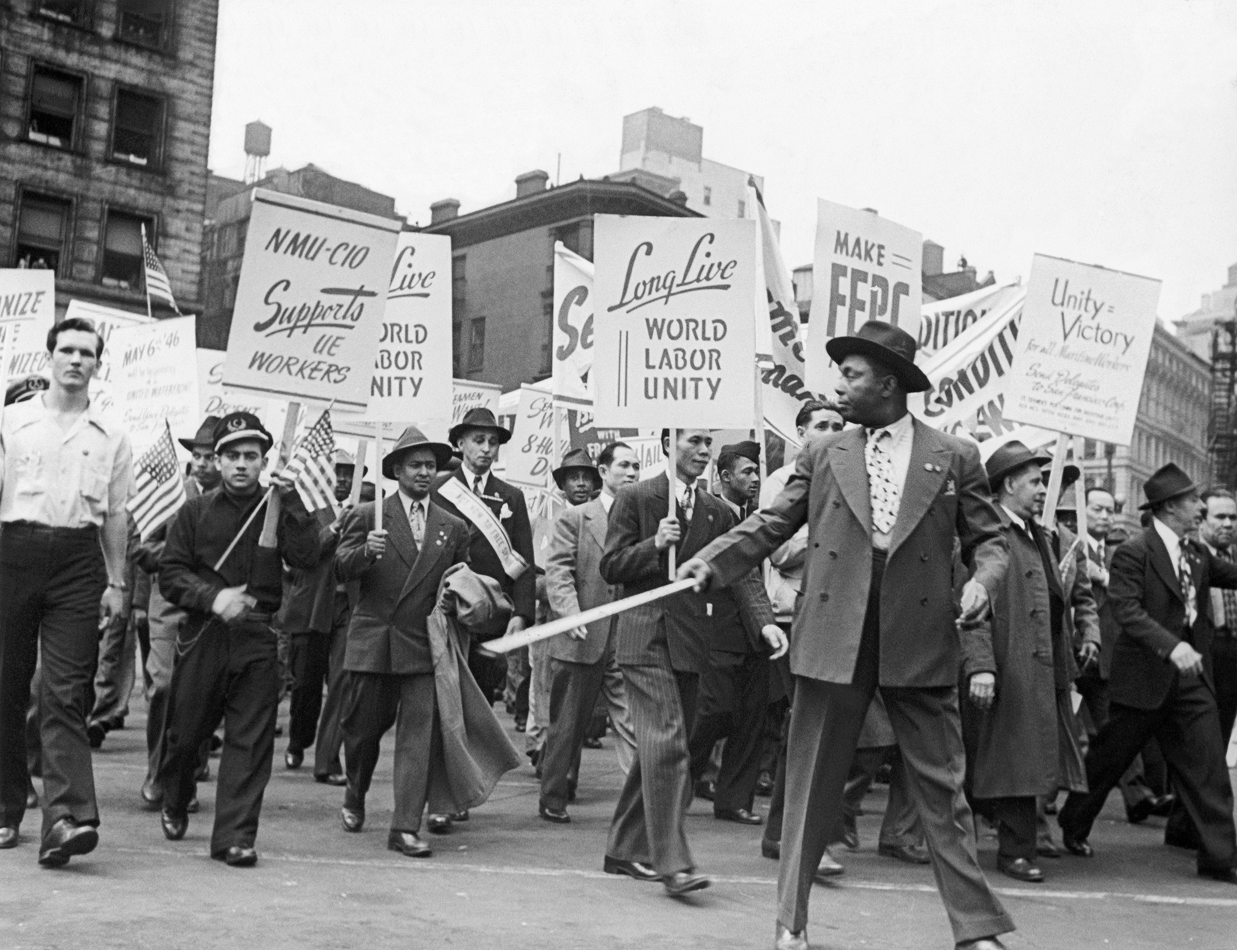
- Diverse workers of various affiliations march together at a 1946 May Day parade in New York City. (Bettmann Archive via Getty Images)
Count this as a post I’ve always wanted to write for myself because I wish I could go back in time to show this to me in graduate school when I was trying (and struggling) to learn Bayesian methods.
If someone were to press me to name my top ten favorite political science articles, assembling and ranking the list would be an ordeal but I can guarantee the reader that Western and Jackman’s (1994) article on Bayesian inference (ungated here) would be in that list. It would be tough to pin down what exactly makes a “great” political science article, the extent to which “favorite” presumably collides with “great” in assembling such a subjective list. The discipline evolves so much. Topics change; for example, few people (to my knowledge) talk about cybneretic decision-making anymore notwithstanding the intellectual currency that topic had in the 1970s to the mid-1980s or so. Methods certainly change. Cheap computing power, coupled with decades of accumulated knowledge, have made the most rudimentary statistical analyses like t-tests, chi-square analyses, and even simple linear models seem like relics. Exceptions include those pushing/advancing experimental designs that largely obviate the need to address thornier selection problems with fancier statistical models. I think the point still remains.
Western and Jackman’s (1994) article would appear on my list with all that in mind largely because it’s the clearest articulation of what Bayesians want and why. The topic is simple but important. The statistical application is clearly simple and others have done more advanced Bayesian analyses, but it was sophisticated for the time. It more importantly served a use clarifying an empirical debate about a topic that was of great scholarly interest in the comparative politics literature at the time and that my undergraduates would already kind of understand jumping into the article cold. It’s why it appears in any quantitative methods class I teach.
While I always understood the basic crux of what the authors were doing, I struggled with a replication of it. The concept of Bayesian inference was simpler for me than the implementation of it. However, the {brms} package has made Bayesian statistical modeling (through Stan) so much simpler. In this case, someone can replicate this article in a matter of minutes.
Some Basic Background
I linked to an ungated version of the Western and Jackman (1994) article article above and I encourage the reader of this post to read that if s/he hasn’t already. It’s well-written and accessible for a college-level audience. Here is a basic synopsis of what Western and Jackman are doing.
Philosophically, two properties of a lot of political science research violate foundations of frequentist inference. First, data of interest are routinely “non-stochastic” and do not follow a random data-generating process. Frequentist inference assumes data are generated by a repeated mechanism (like a coin flip) and that the sample statistic that emerges is just one possible result from a draw of a probability distribution of the population of all results. However, political scientists routinely define the “sample” (and, thus, the sample statistic that emerges) on the population itself. Think of something like wars or Supreme Court decisions. The data are not a sample of the population; they are the population. “Updating” the data doesn’t generate a new random sample; any analysis of war is still going to have World War I in it and any updated analysis of Supreme Court decisions will still have Dred v. Scott and Youngstown Sheet & Tube Company v. Sawyer in it. Frequentist inference is about inferring the likelihood of an extreme sample result given some fixed population parameter of interest. Already so much political science research doesn’t fit this mold, and that’s assuming we know the population parameter of interest (another sticking point for Bayesians).
The second problem Bayesians note is “weak data.” This is maybe a problem of an earlier time. Some political science research, especially comparative politics research of the time interested in advanced countries, had a small number of observations. Basically, if the population of interest is “advanced industrial societies” by 1990, the population had maybe just 24 units in it. Getting a basic statistic of central tendency on 24 units reduces the degrees of freedom to 23. Any other parameters (e.g. regression coefficients) reduces the degrees of freedom further. It’d be asking a lot to do anything with confidence on just 24 observations. The “weak data” problem magnifies another statistical problem: multicollinearity. Multicollinearity is what happens when two predictors on the right-hand side of a regression equation are so highly correlated that their estimated partial effects are uninformative. It’s more likely to happen in a small-n analysis of (largely) similar units.
This all leads to the application for Western and Jackman, and a question of interest to comparative politics scholars of the time. What accounts for the percentage of the work force that is unionized (i.e. union density)? Wallerstein (1989) argues that the primary driver is the size of the civilian labor force. Theoretically, a larger civilian labor force makes collective action that much more difficult, which drives down the percentage of the labor force that’s unionized. Stephens (1991) disputes the primacy that Wallerstein gives to the civilian labor force size. He argues instead that the concentration of the economy in industry is the primary vehicle for labor force size given the unique role that industrialization had as a historical process leading to unionization.
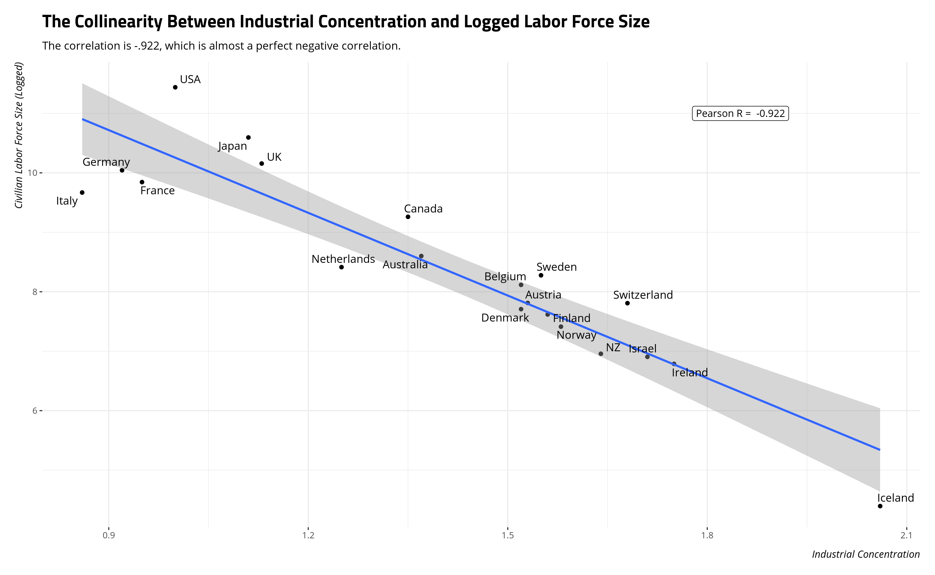
There is a major statistical problem that both authors encounter. Looking at the same basic data (more below) as a cross-section of “advanced industrial societies” of the time, the correlation of civilian labor force size and industrial concentration is over -.9. That’s almost a perfect negative correlation. In many applications, a frequentist model will kick one of the covariates out the model. However, we can still estimate this in a Bayesian model.
The Replication
This replication will depend on just a few packages. {tidyverse} is at the fore of my workflow, followed by my toy {stevemisc} and {stevedata} packages. {stevedata} has the union density data. Finally, the {brms} package will estimate the statistical models. I’m going to use {kableExtra} and {modelsummary} to help format some tables for this blog post. {ggrepel} will appear in a graph. {broom} will do some model processing and {tidybayes} will do some model summaries from {brms} objects.
library(tidyverse)
library(stevemisc)
library(stevedata)
library(brms)
library(kableExtra)
library(modelsummary)
library(ggrepel)
library(broom)
library(tidybayes)
The Data
The data frame is stored in my {stevedata} package as uniondensity. It has 20 rows with four columns. The first column, country, is intuitively the country name. The second column, union, is the dependent variable of interest. It captures the percentage of the work force that is unionized in this cross-section of data. The next column, left, is a control variable of sorts. In other words, Wallerstein and Stephens differ in their competing hypotheses of civilian labor force size and industrial concentration, but agree that left-wing governments have a positive effect on union density. It’s measured from Wilensky’s (1981) cumulative index of left-wing governments, for which the reader will have to go to a university library to find more detail about the measure.
The final two columns are the competing independent variables. size, which is Wallerstein’s “pet” variable of sorts, is the logged civilian labor force size. concen, which is Stephens’ pet variable, is the economic concentration of a country in industry. The data are available in its entirety below.
| country | union | left | size | concen |
|---|---|---|---|---|
| Australia | 51.4 | 33.74 | 8.60 | 1.37 |
| Austria | 65.6 | 48.67 | 7.81 | 1.53 |
| Belgium | 71.9 | 43.25 | 8.12 | 1.52 |
| Canada | 31.2 | 0.00 | 9.26 | 1.35 |
| Denmark | 69.8 | 90.24 | 7.71 | 1.52 |
| Finland | 73.3 | 59.33 | 7.62 | 1.56 |
| France | 28.2 | 8.67 | 9.84 | 0.95 |
| Germany | 39.6 | 35.33 | 10.04 | 0.92 |
| Iceland | 74.3 | 17.25 | 4.39 | 2.06 |
| Ireland | 68.1 | 0.00 | 6.79 | 1.75 |
| Israel | 80.0 | 73.17 | 6.90 | 1.71 |
| Italy | 50.6 | 0.00 | 9.67 | 0.86 |
| Japan | 31.0 | 1.92 | 10.59 | 1.11 |
| Netherlands | 37.7 | 31.50 | 8.41 | 1.25 |
| Norway | 58.9 | 83.08 | 7.41 | 1.58 |
| NZ | 59.4 | 60.00 | 6.96 | 1.64 |
| Sweden | 82.4 | 111.84 | 8.28 | 1.55 |
| Switzerland | 35.4 | 11.87 | 7.81 | 1.68 |
| UK | 48.0 | 43.67 | 10.16 | 1.13 |
| USA | 24.5 | 0.00 | 11.44 | 1.00 |
A careful eye might be able to spot a collinearity problem in the industrial concentration and logged labor force size variables, but a plot will bring it to life.
Setting Priors for the Statistical Models (via Table 1)
The first part of the replication process will set the competing priors into two basic groups: Wallerstein’s priors and Stephens’ priors. Both Wallerstein and Stephens agree on the estimated effect of left-wing governments. So, we set a prior effect of .3 for the beta for left-wing governments with a standard deviation of .15. Both, however, disagree on logged labor force size and industrial concentration. Wallerstein estimates a negative effect of civilian labor force size with a beta of -5 and a standard deviation of 2.5. However, he contends industrial concentration should have zero effect and his priors get a mean of zero with a diffuse standard deviation of 10^6 for that variable. Conversely, Stephens believes logged labor force size has no effect (and thus gets that diffuse/”ignorance” prior) while industrial concentration has an estimated effect of 10 (and a standard deviation of 5). Note, we’ll also set the same diffuse/”ignorance” prior for the intercept even as that might not have been clear from Table 1 in Western and Jackman.
# Wallerstein's priors
# left: 3(1.5)
# size: -5(2.5) // This is what he's arguing
# concen: 0(10^6) // diffuse/"ignorance" prior
# Intercept: 0(10^6) // diffuse/"ignorance" prior
wall_priors <- c(set_prior("normal(3,1.5)", class = "b", coef= "left"),
                 set_prior("normal(-5,2.5)", class = "b", coef="size"),
                 set_prior("normal(0,10^6)", class="b", coef="concen"),
                 set_prior("normal(0,10^6)", class="Intercept"))

# Stephens priors
# left: 3(1.5) // they both agree about left governments
# size: 0(10^6) // diffuse/"ignorance" prior
# concen: 10(5) // This is what Stephens thinks it is.
# Intercept: 0(10^6) // diffuse/"ignorance" prior
stephens_priors <- c(set_prior("normal(3,1.5)", class = "b", coef= "left"),
                     set_prior("normal(0,10^6)", class = "b", coef="size"),
                     set_prior("normal(10,5)", class="b", coef="concen"),
                     set_prior("normal(0,10^6)", class="Intercept"))
Replications with Noninformative Prior Information (Table 2)
Before replicating some of the main results, let’s look at Table 2 of Western and Jackman and see if we can’t replicate that first result. One thing I was astonished to find is the results that Western and Jackman provide in Table 2 aren’t necessarily the result of noninformative prior information. It looks more like it was actually a standard OLS model. Certainly, OLS is giving results identical to what Western and Jackman report. The Stan model estimated in brms is basically identical, but with some slight differences.
# Standard LM
M1 <- lm(union ~ left + size + concen, data=uniondensity)

# Uninformative priors
B0 <- brm(union ~ left + size + concen,
          data=uniondensity,
          # for reproducibility
          seed = 8675309,
          refresh = 0,
          family="gaussian")
#> Running MCMC with 4 chains, at most 8 in parallel...
#>
#> Chain 1 finished in 0.1 seconds.
#> Chain 2 finished in 0.1 seconds.
#> Chain 3 finished in 0.1 seconds.
#> Chain 4 finished in 0.1 seconds.
#>
#> All 4 chains finished successfully.
#> Mean chain execution time: 0.1 seconds.
#> Total execution time: 0.5 seconds.
| Western and Jackman Table 2 | OLS | Bayesian Linear Model | |
|---|---|---|---|
| Left Government | 0.27** | 0.27** | 0.27** |
| (0.08) | (0.08) | (0.08) | |
| Labor Force Size (logged) | −6.46+ | −6.46 | −6.34 |
| (3.79) | (3.79) | (4.18) | |
| Industrial Concentration | 0.35 | 0.35 | 0.69 |
| (19.25) | (19.25) | (21.23) | |
| Intercept | 97.59+ | 97.59 | 96.01 |
| (57.48) | (57.48) | (63.22) | |
| Num.Obs. | 20 | 20 | 20 |
| + p < 0.1, * p < 0.05, ** p < 0.01, *** p < 0.001 |
The basic takeaway from this analysis, as it was in Western and Jackman, is the effects of left-wing governments and logged labor force size are statistically discernible from an argument of zero effect for both predictors. This would make Wallerstein right, prima facie, and make Stephens wrong. Stephens’ industrial concentration variable is insignificant. Indeed, its effect is practically zero.
Incorporating Competing Prior Information (Table 3)
The research question in the Bayesian perspective becomes quite interesting in assessing the analyses conducted and summarized in Table 3. Given the aforementioned “weak” nature of the data, does Wallerstein or Stephens’ respective arguments depend on the prior belief that they are right?
# Wallerstein's priors
B1 <- brm(union ~ left + size + concen,
          data = uniondensity,
          prior=wall_priors,
          seed = 8675309,
          refresh = 0,
          family="gaussian")
#> Running MCMC with 4 chains, at most 8 in parallel...
#>
#> Chain 1 finished in 0.1 seconds.
#> Chain 2 finished in 0.1 seconds.
#> Chain 3 finished in 0.1 seconds.
#> Chain 4 finished in 0.1 seconds.
#>
#> All 4 chains finished successfully.
#> Mean chain execution time: 0.1 seconds.
#> Total execution time: 0.2 seconds.

# Stephens' priors
B2 <- brm(union ~ left + size + concen,
          data = uniondensity,
          prior=stephens_priors,
          seed = 8675309,
          refresh = 0,
          family="gaussian")
#> Running MCMC with 4 chains, at most 8 in parallel...
#>
#> Chain 1 finished in 0.1 seconds.
#> Chain 2 finished in 0.1 seconds.
#> Chain 3 finished in 0.1 seconds.
#> Chain 4 finished in 0.1 seconds.
#>
#> All 4 chains finished successfully.
#> Mean chain execution time: 0.1 seconds.
#> Total execution time: 0.2 seconds.
| Coefficient/Term | Mean | Standard Deviation | Lower Bound | Upper Bound | Prior |
|---|---|---|---|---|---|
| Intercept | 71.49 | 20.66 | 37.27 | 105.53 | Stephens' Priors |
| Intercept | 82.06 | 33.83 | 27.14 | 136.40 | Wallerstein's Priors |
| Left Government | 0.27 | 0.08 | 0.15 | 0.40 | Stephens' Priors |
| Left Government | 0.28 | 0.08 | 0.15 | 0.41 | Wallerstein's Priors |
| Labor Force Size (logged) | -4.84 | 1.86 | -7.86 | -1.74 | Stephens' Priors |
| Labor Force Size (logged) | -5.41 | 2.13 | -8.86 | -1.91 | Wallerstein's Priors |
| Industrial Concentration | 9.28 | 4.79 | 1.34 | 17.37 | Stephens' Priors |
| Industrial Concentration | 4.86 | 13.13 | -16.61 | 26.26 | Wallerstein's Priors |
The results in Table 3, effectively reproduced above, lead to a potentially intriguing implication for this empirical debate. Acknowledging the data are fundamentally weak from the Bayesian perspective, the prior information we build into the models is going to have a lot of influence on the posterior distributions.
The results for the industrial concentration variable are interesting here. Recall, the results in Table 2 suggested the effect of industrial concentration was zero with incredibly diffuse errors. Using Stephens’ priors, we finally observe a significant and positive effect of industrial concentration on union density. But notice, we had to use strong priors to get that result! The results we observed don’t discount the effect of industrial concentration if we build in the prior belief given how weak the data are. In other words, Stephens is correct about the effect of industrial concentration if you build in a strong belief that he should be correct.
The posterior distributions for left governments are unchanged across both priors. Even the effect of civilian labor force size is still discernible from zero in both sets of priors. Only the effect of industrial concentration depends on a prior belief the effect should be there. Ultimately, this lends more support to Wallerstein’s hypothesis than Stephens’ hypothesis.
Conclusion
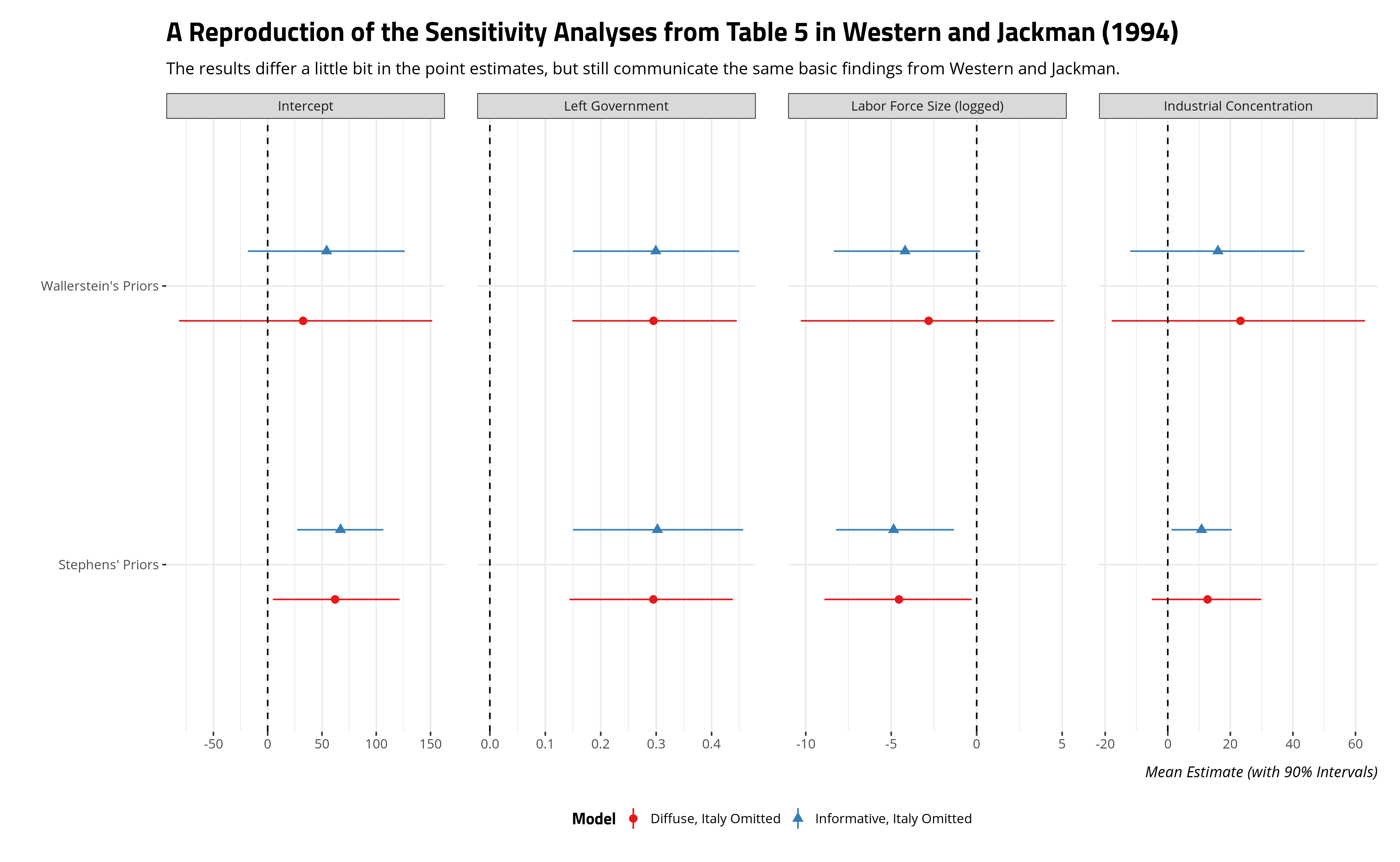
Table 4 and Table 5 in Western and Jackman (1994) do some sensitivity analyses, which 1) omit the outlier case of Italy, and 2) multiply the variances by 10 to diffuse the priors more. The results of those analyses, which I was partially able to replicate, do show the results are sensitive to diffusing the priors. You can see the code for a reproduction of the same basic findings from Table 5 below.
# The sensitivity analyses are:
# 1) keep the informative priors, but exclude Italy
# 2) multiply the variances by 10, and exclude Italy.
#    Notice: variances. Take sd to power 2, then multiply by 10, then sqrt()

wall_priors_diffuse <- c(set_prior("normal(3, sqrt(3*10))", class = "b", coef= "left"),
                         set_prior("normal(-5, sqrt(5*10))", class = "b", coef="size"),
                         set_prior("normal(0,10^6)", class="b", coef="concen"),
                         set_prior("normal(0,10^6)", class="Intercept"))

stephens_priors_diffuse <- c(set_prior("normal(3, sqrt(3*10))", class = "b", coef= "left"),
                         set_prior("normal(0,10^6)", class = "b", coef="size"),
                         set_prior("normal(10,sqrt(10*10))", class="b", coef="concen"),
                         set_prior("normal(0,10^6)", class="Intercept"))

B3 <- brm(union ~ left + size + concen,
          data = subset(uniondensity, country != "Italy"),
          seed = 8675309,
          refresh = 0,
          prior=wall_priors,
          family="gaussian")
#> Running MCMC with 4 chains, at most 8 in parallel...
#>
#> Chain 1 finished in 0.1 seconds.
#> Chain 2 finished in 0.1 seconds.
#> Chain 3 finished in 0.1 seconds.
#> Chain 4 finished in 0.1 seconds.
#>
#> All 4 chains finished successfully.
#> Mean chain execution time: 0.1 seconds.
#> Total execution time: 0.2 seconds.

B4 <- brm(union ~ left + size + concen,
          data = subset(uniondensity, country != "Italy"),
          seed = 8675309,
          refresh = 0,
          prior=wall_priors_diffuse,
          family="gaussian")
#> Running MCMC with 4 chains, at most 8 in parallel...
#>
#> Chain 1 finished in 0.1 seconds.
#> Chain 2 finished in 0.1 seconds.
#> Chain 3 finished in 0.1 seconds.
#> Chain 4 finished in 0.1 seconds.
#>
#> All 4 chains finished successfully.
#> Mean chain execution time: 0.1 seconds.
#> Total execution time: 0.2 seconds.


B5 <- brm(union ~ left + size + concen,
          data = subset(uniondensity, country != "Italy"),
          seed = 8675309,
          refresh = 0,
          prior=stephens_priors,
          family="gaussian")
#> Running MCMC with 4 chains, at most 8 in parallel...
#>
#> Chain 1 finished in 0.1 seconds.
#> Chain 2 finished in 0.1 seconds.
#> Chain 3 finished in 0.1 seconds.
#> Chain 4 finished in 0.1 seconds.
#>
#> All 4 chains finished successfully.
#> Mean chain execution time: 0.1 seconds.
#> Total execution time: 0.2 seconds.

B6 <- brm(union ~ left + size + concen,
          data = subset(uniondensity, country != "Italy"),
          seed = 8675309,
          refresh = 0,
          prior=stephens_priors_diffuse,
          family="gaussian")
#> Running MCMC with 4 chains, at most 8 in parallel...
#>
#> Chain 1 finished in 0.1 seconds.
#> Chain 2 finished in 0.1 seconds.
#> Chain 3 finished in 0.1 seconds.
#> Chain 4 finished in 0.1 seconds.
#>
#> All 4 chains finished successfully.
#> Mean chain execution time: 0.1 seconds.
#> Total execution time: 0.2 seconds.
The point estimates differ a little but the same basic story emerges that emhasize the effect of diffuse priors on low-n statistical analysis even if the implications appear greater for Stephens’ hypothesis. Indeed, omitting Italy and using Stephens’ priors produces stronger evidence for the effect of civilian labor force size than Wallerstein’s prior when Italy is omitted. Generally, sensitivity analyses highlight the importance of priors when data are weak.
Still, this post is a love letter of sorts to the Western and Jackman (1994) article and to the {brms} package for doing Bayesian statistical modeling with the Stan programming language. The article appears on every quantitative methods syllabus of mine and {brms} is an incredibly useful tool for getting standard R users to do more Bayesian modeling. You can use the latter to replicate the statistical analyses in the former, which might help the learning experience for students trying to unpack Western and Jackman’s research design.
Disqus is great for comments/feedback but I had no idea it came with these gaudy ads.