Mixed Effects Modeling Tips: Use a Fast Optimizer, but Perform Optimizer Checks

The R logo, just 'cause.

Last updated: 26 August 2021. The data can be more easily loaded in {stevedata} as the wvs_usa_abortion data frame. The results will be slightly different as well. I’ve also added a simulation of 100 trials for each optimizer.

My goals for writing this are two-fold. First, it’d been a long time since my last blog post. I usually average 7-10 posts a year and this will only be the second one. Second, I’ve been meaning to offer some tips/tutorials for mixed effects modelers who are still new to the craft. Mixed effects modeling is my method of choice for evaluating and explaining social/political phenomenon. I think I’ve become pretty good at it over the past 10 years, but everything I know I ultimately taught myself through trial and error. Stackoverflow is nice but I was always reticent to post there to search for answers I feel I should’ve known already. It does mean that while I everything I know is self-taught, I’ve learned a lot of tricks along the way and I think it would be good to share them.

Here, I start what might be a series of similar posts with one of the nagging issues of mixed effects modeling: computation time. Computation time can drag in the mixed effects modeling framework in R because {lme4}, the most popular mixed effects modeling tool in R, performs a myriad of convergence checks that can drag on forever. Modeling several hundred thousand observations (like I routinely do with the World Values Survey) can compound the problem.

Here, I offer some tips on how to make the most computation times by selecting the fastest optimizer and, importantly, benchmarking the fast optimizer you choose against a series of different optimizers using the allFit() function. I will start with the R packages I’ll be using in this post before describing the data.

library(tidyverse) # for most things
library(stevemisc) # helper functions/formatting
library(stevedata) # the data
library(lme4) # for mixed models
library(broom.mixed) # for mixed model tidiers

A Brief Description of the Data

We’ll start with a toy data set I created from six waves of American responses in the World Values Survey for my quantitative methods class. This data set probes attitudes toward the justifiability of an abortion, a question of long-running interest to “values” and “modernization” scholarship. It appears in the surveys the World Values Survey administered in 1982, 1990, 1995, 1999, 2006, and 2011. The variable itself is coded from 1 to 10 with increasing values indicating a greater “justifiability” of abortion on this 1-10 numeric scale. I’ll offer two dependent variables below from this variable. The first will treat this 1-10 scale as interval and estimate a linear mixed effects model on it. This is problematic because the distribution of the data would not satisfy the assumptions of a continuous and normally distributed dependent variable, but I would not be the first person to do this and I’m ultimately trying to do something else with this exercise. The second will condense the variable to a binary measure where 1 indicates a response that abortion is at least somewhat justifiable. A zero will indicate a response that abortion is never justifiable.

I’ll keep the list of covariates simple. The models include the respondent’s age in years, whether the respondent is a woman, the ideology of the respondent on a 10-point scale (where increasing values indicate greater ideology to the political right), how satisfied the respondent is with her/his life on a 10-point scale, the child autonomy index (i.e. a five-point measure where increasing values indicate the respondent believes children should learn values of “determination/perseverance” and “independence” more than values of “obedience” and “religious faith”), and the importance of God in the respondent’s life on a 1-10 scale. The point here is not to be exhaustive of attitudes about abortion in the United States, but to provide something simple and intuitive for another purpose.

You can see the exact code I’m using below, along with the rescaling I do.

wvs_usa_abortion %>%
  mutate(ajd = carr(aj, "1=0; 2:10=1")) %>%
  # r2sd_at() is in {stevemisc}
  r2sd_at(c("age", "ideology", "satisfinancial", "cai", "godimportant")) -> Data

M1 <- lmer(aj ~ z_age + female + 
             z_ideology + z_satisfinancial + z_cai + z_godimportant + 
             (1 | year), data = Data,
           control=lmerControl(optimizer="bobyqa",
                                 optCtrl=list(maxfun=2e5)))
M2 <- glmer(ajd ~ z_age + female + 
             z_ideology + z_satisfinancial + z_cai + z_godimportant + 
              (1 | year), data = Data, family=binomial(link="logit"),
            control=glmerControl(optimizer="bobyqa",
                                 optCtrl=list(maxfun=2e5)))

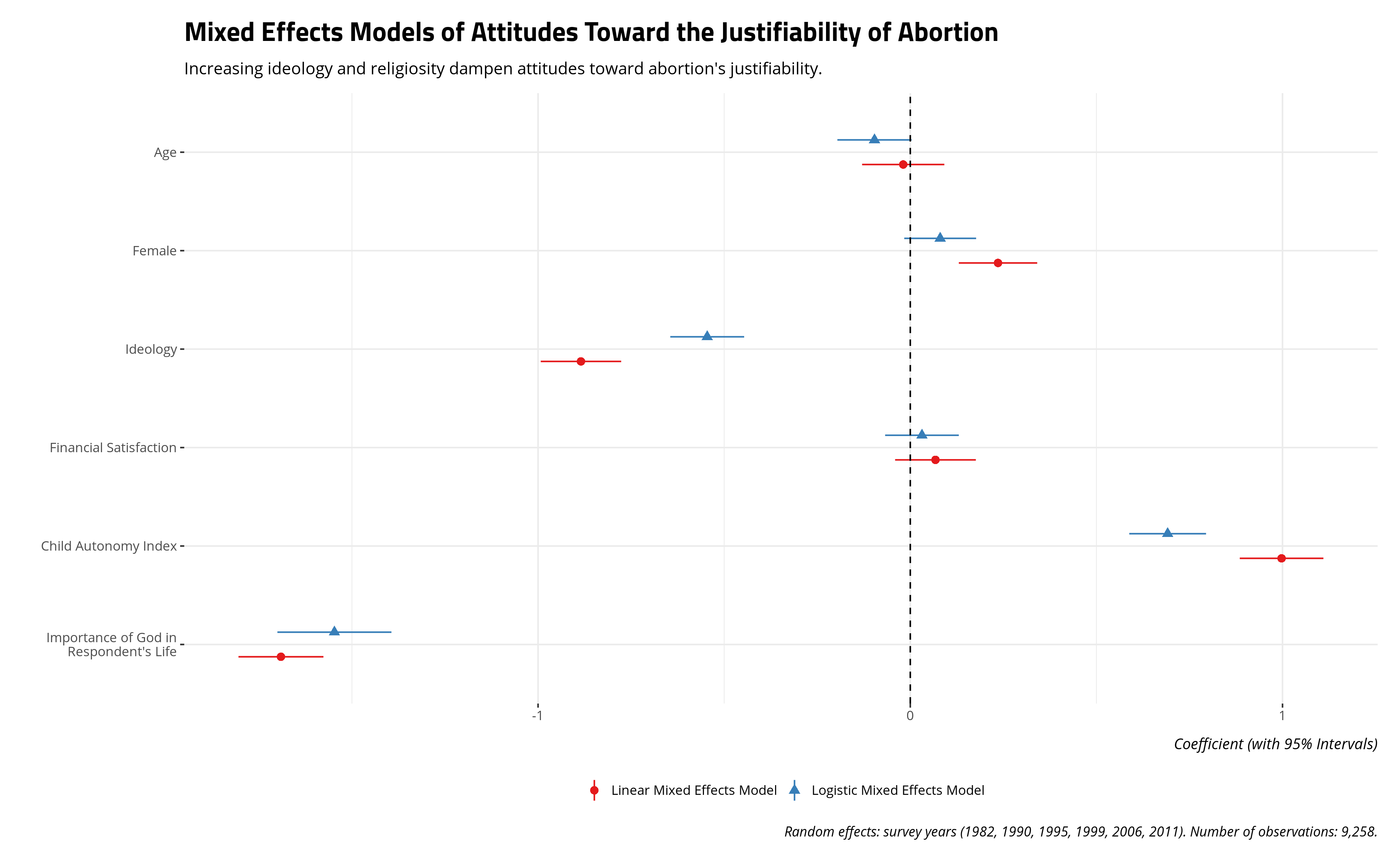
I provide the results below with my optimizer of choice. I am partial to bound optimization by quadratic approximation (BOBYQA) with a set maximum of 200,000 iterations (BOBYQA recommends at least 100,000). I do this because I’ve found, in my experience, this optimization to be a nice medium between speed and a valid convergence. It rarely gives me convergence warnings and, in the rare event that it does, it almost never provides parameter estimates that would differ much from other forms of convergence.

The results below are substantively intuitive. Age might have a negative effect on attitudes toward abortion, but we see that in the logistic model and not the linear model. It should be unsurprising that increasing ideology to the right and increasing religiosity (i.e. the importance of God in the respondent’s life) decrease attitudes toward abortion’s justifiability. The child autonomy index has a positive effect on the justifiability of abortion, which is consistent with received wisdom from “modernization” and “values” scholarship.

Performing Optimizer Checks

You can conveniently refit your statistical model with multiple different optimizers using the allFit() function, which you can import from the {lme4}. I’ll briefly summarize these optimizers below.

The standard generalized linear mixed effects model estimation does parameter optimization through a combination of BOBYQA and the Nelder-Mead “downhill simplex” method. This approach is “standard” for estimation but, in practice, creates much longer computation times as the optimization goes through a series of convergence checks. It’s understandable for a precaution; sometimes the model needs these convergence checks and the researcher should know the results of these convergence checks. However, it can create a wait for your results and it may not matter, contingent on the model you estimate.

allFit() will test whether your optimization choice you make for convenience may change the results of the model. It will re-estimate your model with a series of different optimizers. These are the aforementioned Nelder-Mead method and the BOBYQA method. It’ll use those same optimizers, but permit additional stopping criteria through non-linear optimization (nlopt) if the optimization procedures believes it has found the optimum. This speeds up computation at the expense of additional convergence checks. Additional optimization methods include large-scale, quasi-Newton, bound-constrained optimization of the Byrd et al. (1995) method (L-BFGS-B), iterative derivative-free k-bounded optimization of the Nelder-Mead method (nmkb), and non-linear minimization with box constraints (nlminb). My worry is I forgot one of these optimizers that allFit() has, so these are the optimizers with which I’m most familiar.

Here’s how you would perform these additional optimizer checks in my sample analysis. Do note that {lme4} only “suggests” and does not “import” the {optimx} and {dfoptim} packages. Both are necessary for the allFit() function, so make sure to install those. If you have them installed, {lme4} will load them both when you call this function.

AF1 <- allFit(M1, verbose=F)
AF2 <- allFit(M2, verbose=F)

You can leverage allFit() in multiple ways. First, it would be useful information for the appendix of your paper, should you choose the fastest optimizer you want at the expense of multiple and potentially redundant convergence checks, to report the log-likelihoods of the various models that allFit() estimated. I do this graphically below.

AF1_lliks <- sort(sapply(AF1,logLik))
AF2_lliks <- sort(sapply(AF2,logLik))

bind_rows(AF1_lliks, AF2_lliks) %>%
  remove_rownames(.) %>%
  mutate(model = c("Linear Mixed Effects Model", "Logistic Mixed Effects Model")) %>%
  select(model, everything()) %>%
  group_by(model) %>%
  gather(., Optimizer, llik, 2:ncol(.)) %>%
  ggplot(.,aes(Optimizer, llik)) + geom_point() +
  facet_wrap(~model) + coord_flip() +
  theme_steve_web() +
  ylab("Log-Likelihood") +
  labs(title = "The Log-Likelihoods of Seven Different Optimizers in Our Two Models")

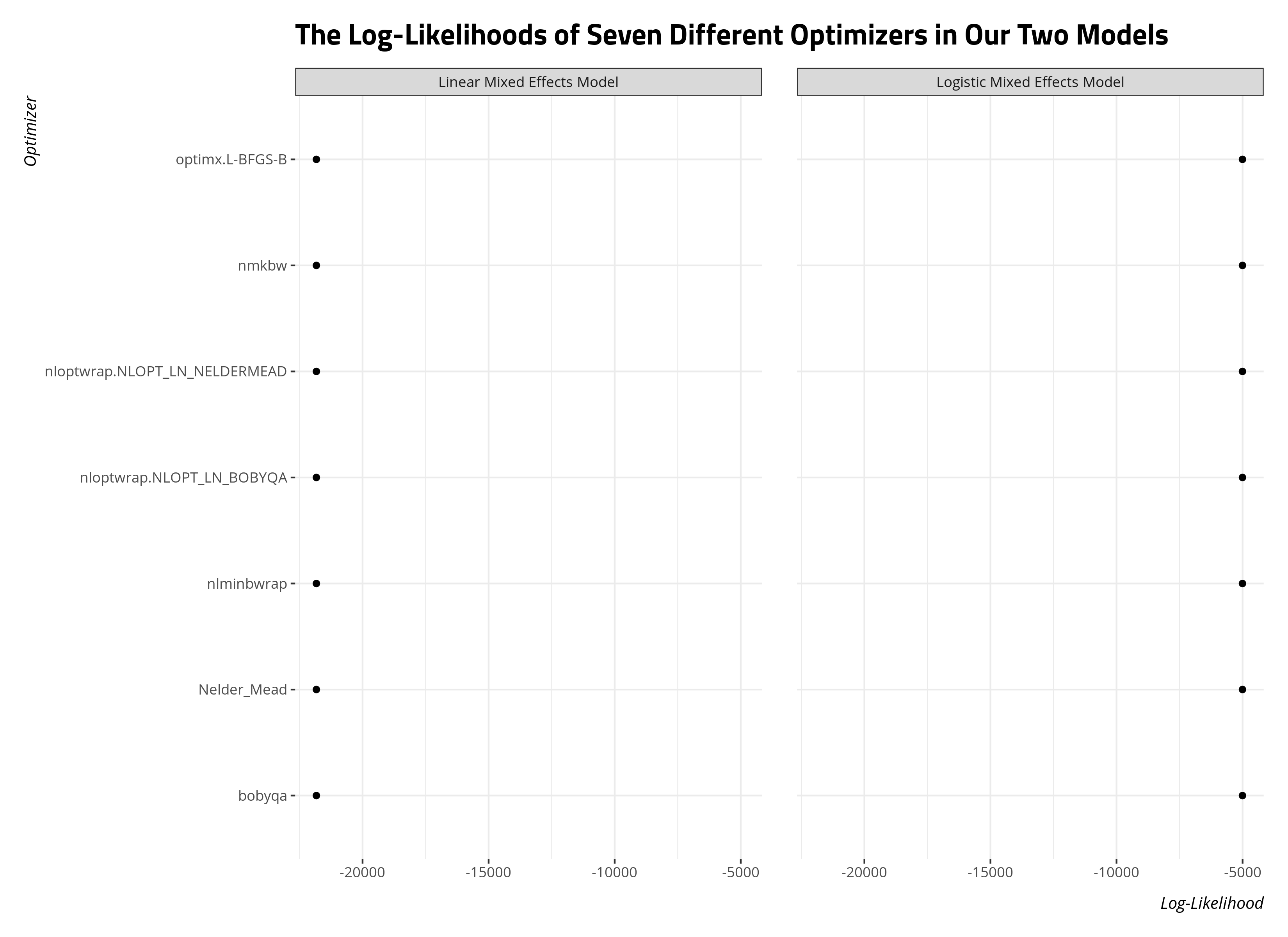
The easiest way to interpret this is that these log-likelihoods should all be within thousandths of a decimal point from each other. The optimizer does not influence the parameter estimates if these facets all have dots in a single column like this. Here, we can be assured that the model’s parameters we report do not depend on the optimizer we chose.

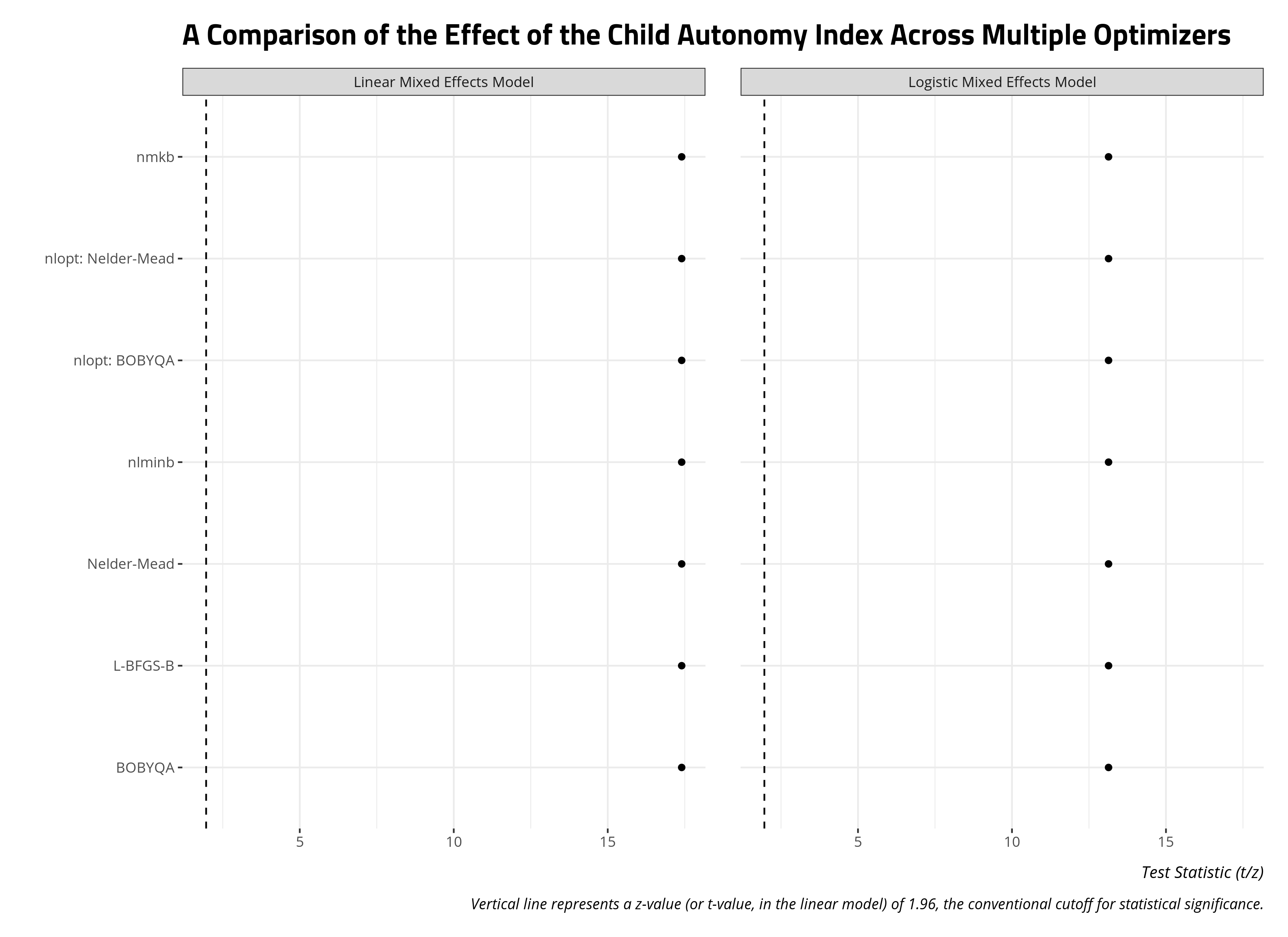
You could also do something similar with the z-statistics and t-statistics of a particular variable from the model. Let’s assume I’m interested, for theoretical reasons, in the effect of the child autonomy index on attitudes toward abortion in my model. I’m trying to build an argument about this relationship we observe and demonstrate to reviewers that the effect is not sensitive to the optimizer. Toward that end, I can pool all the coefficients for the child autonomy index variable across all the optimizers and present them as a faceted plot like above. The intuition here is straightforward, as it was above. If the points on the plot below all form a single column across both facets, then the parameter for the variable is robust to the particular optimizer.

lapply(AF1, tidy) %>%
  map2_df(.,
          names(AF1),
          ~mutate(.x, optimizer = .y)) %>%
  filter(term == "z_cai") %>%
  mutate(optimizer = c("BOBYQA", "Nelder-Mead",
                       "nlminb", "nmkb",
                       "L-BFGS-B",
                       "nlopt: Nelder-Mead",
                       "nlopt: BOBYQA")) %>%
  mutate(Model = "Linear Mixed Effects Model") -> AF1_zcai

lapply(AF2, tidy) %>%
  map2_df(.,
          names(AF2),
          ~mutate(.x, optimizer = .y)) %>%
  filter(term == "z_cai") %>%
  mutate(optimizer = c("BOBYQA", "Nelder-Mead",
                       "nlminb", "nmkb",
                       "L-BFGS-B",
                       "nlopt: Nelder-Mead",
                       "nlopt: BOBYQA")) %>%
  mutate(Model = "Logistic Mixed Effects Model") -> AF2_zcai

bind_rows(AF1_zcai, AF2_zcai) %>%
  ggplot(.,aes(optimizer, statistic)) + geom_point() +
  theme_steve_web() +
  coord_flip() + facet_wrap(~Model) +
  geom_hline(yintercept = 1.96, linetype="dashed") +
  labs(caption = "Vertical line represents a z-value (or t-value, in the linear model) of 1.96, the conventional cutoff for statistical significance.",
       title = "A Comparison of the Effect of the Child Autonomy Index Across Multiple Optimizers",
       x = "", y = "Test Statistic (t/z)")

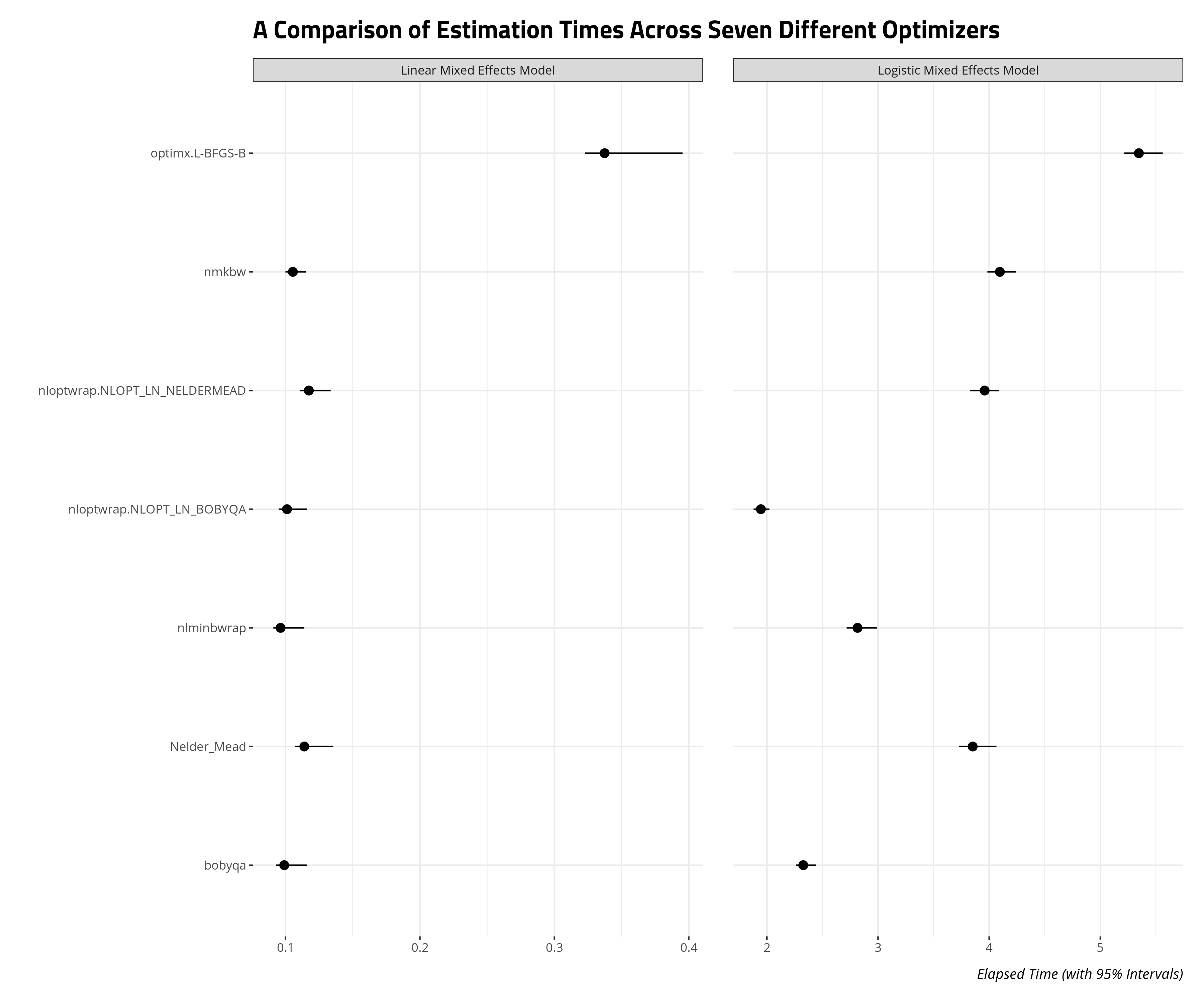
allFit() will helpfully store the estimation times of these models as well. This will be useful as you figure out which optimizer gives you the most “bang for your buck” (i.e. what converges the fastest, especially if you’re short on memory and time). I devised a script that estimated these two models, and re-fitted them with allFit() 100 times. The data that emerged is the elapsed run time for each optimizer across 100 iterations.

The results suggest you can get the most bang for your buck through non-linear optimization of the BOBYQA method or the BOBYQA method itself. The non-linear optimization result is unsurprising because this procedure permits stopping convergence checks earlier if it believes it has already found an approximate optimum. The differences may not matter as much for linear models in the mixed effects framework. These already estimate quickly, all things considered. No matter, BOBYQA might be the way to go if you want a quick and honest look at the results of your logistic mixed effects model.

Conclusion

Optimizer performance is an advanced topic for those fluent in the mixed effects modeling framework in R. However, it’s useful information for beginners as they explore model estimation and, importantly, want to estimate as many models as they can within as short of a time as possible.

It’s useful for researchers to take advantage of the allFit() function in R, at least as a robustness check for the appendix of the paper. You can use this wrapper function to re-estimate the statistical model with multiple optimizers to see if the log-likelihoods of the model chosen for presentation is sensitive to the particular optimizer of the model. The researcher can also compare z/t statistics for a particular coefficient across multiple optimizers. A researcher just learning about the mixed effects modeling framework can also use the allFit() function to identify what optimizers converge the fastest. If you’re like me, who learned mixed effects models by estimating hundreds of models just to see how the process worked, this is useful information. You don’t need to be advanced in the method to appreciate it.