Simulate Time Series Diagnostics with {sTSD}

You don't have to treat critical values from non-standard distributions as gospel in this day and age. See them for yourself.

I’m writing this for an advanced quantitative methods class I teach in our Master’s program in the Department of Economic History and International Relations. A department of two somewhat disparate disciplines, the curriculum we have at the Master’s level endeavors to teach students interested in both basic disciplines at a foundation level. That concerns the quantitative methods sequences (in which I feature prominently) and concerns time series topics (which feature more in quantitative economic history and not international relations as much). Thus, moving here meant I needed to teach myself some things I had never needed to learn before as either part of my methods training or as a tool for some project I was doing.

Enter the wonderful world of unit root testing, a common procedure for time series analyses where a vector (time series) does not hover around some constant mean. If this describes your data—and it sure as hell describes just about any series that you might be watching on Yahoo Finance—then a failure to adequately diagnose it could lead you down a path to a slew of errors. You have multiple options for how you might diagnose so-called “non-stationarity” or “unit roots”,¹ but the classic one is the Dickey-Fuller test. There is no shortage of packages available for doing unit root tests in R. The familiar {tseries} will do it, as will {urca} and {aTSA} (among many others, I’m sure). All work for what they’re intended to do, but all will make evident one of the more whimsical/frustrating things about this procedure. It’s a test that produces a p-value, for which there is a null hypothesis, but it references a non-standard distribution whose critical values themselves were once simulated over 50 years ago on a Canadian super computer of its time. The end result leaves the baffled student and the professor teaching himself this procedure imagining themselves in the crowd while Moses returns with the 10 (or 15) commandments. “Interesting. Makes sense? But you’re leaving me wanting to see this for myself.”

When you understand what it’s doing, it really takes no effort to do this yourself. The R package I wrote to do this, {sTSD}, handles the (Augmented) Dickey-Fuller test and related Phillips-Perron and Kwiatkowski et al. (KPSS) procedures in the same way.² It takes an assumed time series you give it and simulates some user-specified number of time series that matches it description, either stationary or non-stationary.

Here are the R packages that will appear in this post.

library(tidyverse)   # for most things...
library(stevethemes) # for my themes/themeing elements
library(sTSD)        # the star of the show
library(ggh4x)       # for a more flexible nested plot element in {ggplot2}

Here’s a table of contents.

1. What Are These Unit Root Tests Trying to Accomplish?
2. About That t-Statistic, Though…
3. What {sTSD} Does
4. See It For Yourself, with an Applied Example
5. Conclusion

What Are These Unit Root Tests Trying to Accomplish?

I get the basis of this question from watching an interview with Bradley Efron in 2014, where he discusses the origin of the bootstrap as a question about what its predecessor (the jackknife) was trying to accomplish. Every statistical procedure is trying to accomplish something with some question or problem in mind. The Dickey-Fuller test, its augmented form, and its successors (Phillips-Perron, KPSS) are no different.

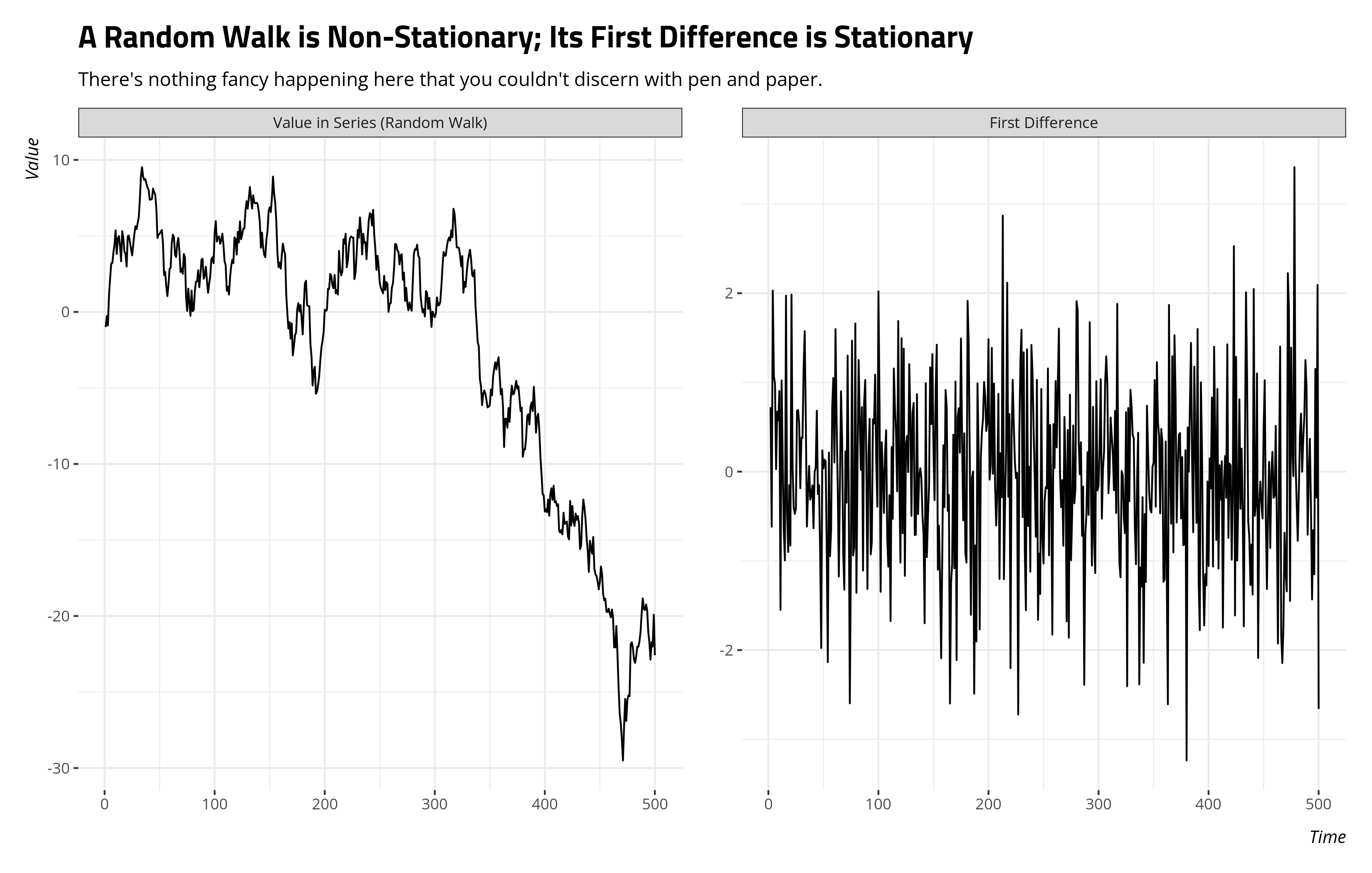
We know that non-stationarity poses considerable problems for statistical inference and joint non-stationarity may even lead to problems of spurious regression. What procedure might warn us of these potential issues? Consider the case of the simple random walk, where the observation of y at time point t is a function of its previous value and some random shock/error. We’d express this form as follows.

This coefficient (\(\rho\)) communicates the kind of memory in the series and has an assumed bound between 0 and 1. If \(\rho\) is 0, there is no memory whatsoever in the series and the series itself becomes basic noise over time. If \(\rho\) is 1, there is lasting memory in the series. Sometimes likened to a “drunkard’s walk”, the series has a critical path dependence like a drunkard stumbling out of the bar and toward nowhere in particular. There is randomness, but each “step” along the way is maximally dependent on the steps (and previous randomness) before it.

Conceptualizing a way out of this doesn’t take too much effort. It only takes a simple pen and the nearest available piece of paper or napkin. Start by subtracting the previous observation (\(y_{t-1}\)) from the current observation (\(y_t\)) and you get the familiar difference term (\(\Delta y_t\)). If you understand that the previous observation (\(y_{t-1}\)) is unweighted with a value of 1, you get this derivation and the introduction of a new coefficient (\(\gamma\)) to summarize this relationship.

The formula syntax may not be welcome for beginners, but the principle is pretty straightforward. A maximally autoregressive series (\(\rho\) = 1) is, we would say, first-difference stationary on paper. When this is true, \(\gamma\) (or \(\rho - 1\)) is 0 and the previous value should tell you absolutely nothing about the change in the current value from the previous value. Only \(e_t\) remains to account for the difference in a series with total information retention.

Simulation by way of fake data shows how this works. After setting a reproducible seed, we’ll create a simple series of 500 time units. Then, we’ll generate random noise (e) and allow the outcome (y) to be the cumulative sum of this random noise. Whereas the cumulative sum maximally weights the previous observation, and by extension all those before it, this is the pure random walk. The first difference of this (d_y) returns us just the noise at the expense of the first observation in the series.

set.seed(8675309) # Jenny, I got your number...
tibble(t = 1:500, # 500 time units
       e = rnorm(500), # 500 random numbers
       y = cumsum(e),  # the random walk, then...
       # the first difference.
       d_y = y - lag(y)) -> fakeWalk

fakeWalk # let's see the data
#> # A tibble: 500 × 4
#>        t       e      y     d_y
#>    <int>   <dbl>  <dbl>   <dbl>
#>  1     1 -0.997  -0.997 NA     
#>  2     2  0.722  -0.275  0.722 
#>  3     3 -0.617  -0.892 -0.617 
#>  4     4  2.03    1.14   2.03  
#>  5     5  1.07    2.20   1.07  
#>  6     6  0.987   3.19   0.987 
#>  7     7  0.0275  3.22   0.0275
#>  8     8  0.673   3.89   0.673 
#>  9     9  0.572   4.46   0.572 
#> 10    10  0.904   5.37   0.904 
#> # ℹ 490 more rows

Here’s what a plot of these data would look like.

What happens when we lose this kind of “memory” in the series? In any instance where \(\rho\) < 1, \(\gamma\) in the above equation is necessarily negative. Thus, the past observation starts to tell you something about the next period’s change through a correction mechanism or mean reversion. Past values above the mean in \(y\) get “corrected” and pull down to the mean of the overall series. Past values below the mean in \(y\) get corrected and pull up to the mean of the overall series. Again, referenced to the above formula, \(\gamma\) is negative. Referenced to some kind of linear model of this mechanism, the t-statistic you get predicting the current period’s change with the last observed value will come back more negative than it would in the pure random walk. There’s a correction, and we can feel more “confident” predicting such a correction in the presence of even partial memory. Observe in the case where \(\gamma\) is -.5 (i.e. \(\rho\) in arima.sim() is .5).

tibble(t = 1:500,
       y = as.vector(arima.sim(n = 500, list(ar = 0.5), sd = 1)), 
       d_y = y - lag(y)) -> fakeAR

# Compare the pure random walk...
summary(M1 <- lm(d_y ~ 0 + lag(y), fakeWalk))$coefficients
#>            Estimate  Std. Error     t value  Pr(>|t|)
#> lag(y) 3.886658e-05 0.004867894 0.007984272 0.9936327

# ...with one that has partial memory.
summary(M2 <- lm(d_y ~ 0 + lag(y), fakeAR))$coefficients
#>          Estimate Std. Error   t value     Pr(>|t|)
#> lag(y) -0.4842694 0.03804168 -12.72997 2.457904e-32

The past value tells you nothing of the current value’s change in the random walk, but it tells you a lot in the case where memory is just partial and the series corrects to its mean. That predictive power is communicated in the t-statistic of a simple linear model.

About That t-Statistic, Though…

It would be ideal if that t-statistic of the model were sufficient for making inferential claims, but it isn’t. That is indeed the test statistic of note, but the statistic doesn’t follow the inferential process of the simple linear model because the test is over the residual term and not the raw data of the series. Instead, we need some other set of critical values for making inferential claims about non-stationarity in the time series. Enter the following table, which first appeared in either Fuller (1976) or Dickey (1976). I have Dickey’s (1976) dissertation, if not Fuller’s (1976) textbook, so I’ll present the Dickey (1976) version.

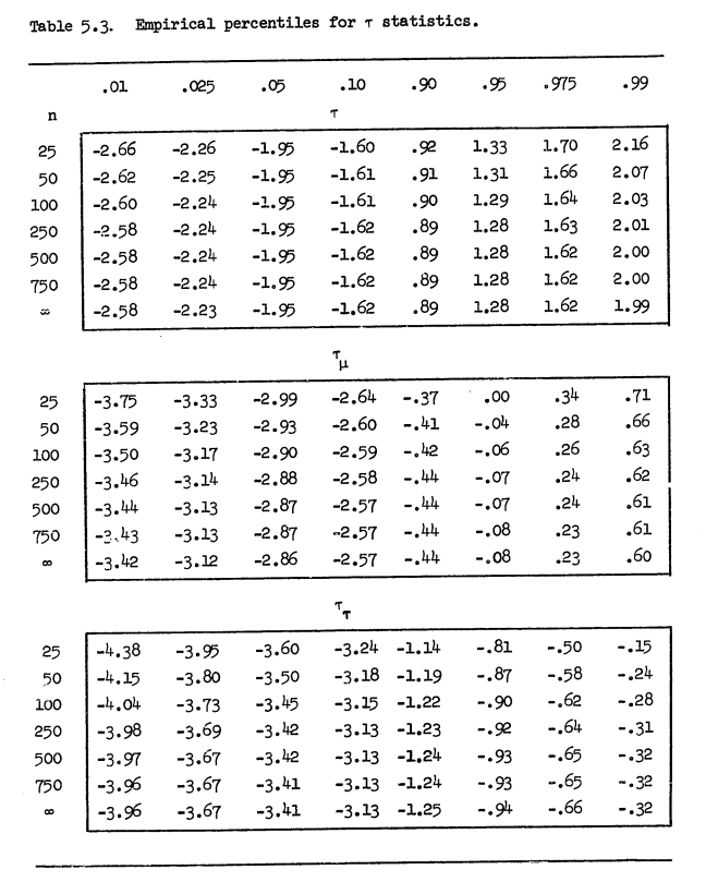
Critical Values of the Dickey-Fuller Test, by Way of Dickey (1976)

For added context, these values are the product of an extensive Monte Carlo simulation carried out with assistance from a supercomputer at McGill University at the time (“Super Duper”). Assume a standard normal distribution (with a mean of 0 and a standard deviation of 1). Now, prepare (in the table’s case) a vector of length 25, 50, 100, 250, 500, 750, and \(\infty\).³ Further assume the pure random walk from the aforementioned standard normal distribution and related data-generating processes for which there is a y-intercept (i.e. a “drift”, in time series parlance) and a linear time trend that increments by 1 across the length of the vector. For each of those vectors corresponding with those data-generating processes, replicate the procedure on these vectors anywhere from 10,000 to 100,000 times. Get the t-statistics for each of those as a kind of distribution of test statistics under the assumption of a non-stationary time series (because they’re random walks). Break those into percentiles corresponding with anywhere from 1% to the 99%. Recall that the test statistics are intended to come back negative for real-world cases, so we should focus our attention on those magic numbers like .05 or .10 corresponding with the left tail.

Enter one of the first frustrating features of this procedure: the null hypothesis. This is one of those procedures. The null hypothesis here is clumsily stated as equivalent to “problem”, in contrast with other diagnostic tests like Breusch-Pagan, Breusch-Godfrey, and Durbin-Watson (in which the null hypothesis is “no problem”). If the test statistic is less than (“more negative than”) one of those critical values of your choice, you can reject the null hypothesis of “problem” (i.e. non-stationarity) and instead accept the alternative hypothesis of “no problem” (i.e. stationarity). If you cannot reject the null hypothesis, you have a problem. However, you’re making a statement of compatibility or incompatibility of the null hypothesis referencing various distributions that are almost assuredly not your own. You’re further making assessments of your ability to reject the null hypothesis against a distribution that is somewhat parked only when the time series you have is not stationary. That’d be the rationale for “problem” as the null hypothesis. If your time series is stationary, the distribution of plausible statistics moves contingent on \(\rho\) and how long the series is.

This test is a case where the logic is nifty but the execution has left me a bit wanting ever since I had to start teaching about this procedure. For one, literally every textbook reproduces this exact table from either Fuller’s (1976) textbook or Dickey’s (1976) dissertation. I don’t doubt the output of the model, but its utility is defined by implicit assumptions in a 50-year-old supercomputer and the multiple other assumptions Dickey and Fuller built into the procedure. Two, much like anything involving a t-statistic, it is never offered in relation to your actual data. I will never have a data set of 25, 50, 100, 250, 500, 750, or \(\infty\) observations, so what these statistics mean for my time series of 336 observations or 83 observations has to be approximated or interpolated through other means. This makes it kind of biblical, in a way. It’s again similar to Moses coming down on high with ten commandments ad infinitum without any real means to square ten simple dictates with the exigencies of real life. The third complaint isn’t really the fault of anyone in particular, but this function is non-standard. Summary by simulation was the only way to go and Dickey and Fuller do at least provide an honest framework based on simulation that very few people could do 50 years ago. But I can do this now.⁴ All of us have better technology than Dickey and Fuller had 50 years ago. Why not? It would certainly circumvent some of the awkwardness of doing inference by the null hypothesis. It’s non-standard anyway, so why do it this way when I can simulate based on features about my time series instead (rather than the standard normal distribution).

What {sTSD} Does

{sTSD} is born from my frustration with these procedures, and also my affinity for simulating things. sadf_test(), which handles both the Dickey-Fuller and its “augmented” corollary, looks like this.

sadf_test(x, n_lags = NULL, n_sims = 1000, sim_hyp = "nonstationary")

sadf_test() takes a vector of an assumed time series (x). It then asks for some number of simulations (n_sims) you would like to do, with a default of 1,000. Thereafter, it will simulate the user-specified number of simulations from either a pure white noise time series (sim_hyp = 'stationary') or three different time series (sim_hyp = 'nonstationary') where the data are either a pure random walk, a random walk with a drift (y-intercept), or a random walk with a drift and trend (i.e. y-intercept and time trend). It then runs the Dickey-Fuller or its “augmented” version on all those simulated series, contingent on what you provide to the n_lags argument in the function.⁵ It will allow you to assess whether your time series is stationary or non-stationary by comparison to simulated series of the exact length of your series that is known to be stationary or non-stationary in some form.

Let’s do a simple Dickey-Fuller test (n_lags = 0) with just 100 simulations to make this quick, and to explore its basic output. The output will come back as a list with a specialty class provided by the function.

DF1 <- sadf_test(fakeWalk$y, n_lags = 0, n_sims = 100)
class(DF1)
#> [1] "sadf_test"
names(DF1)
#> [1] "stats"      "sims"       "attributes"

The first element, ("stats"), is the test statistics. In order, they are the test statistic for the Dickey-Fuller test with 1) no drift nor trend, 2) drift, no trend, and 3) drift and trend. You can compare with it communicates with the corollary functions in the {urca} and {aTSA} package.

DF1$stats
#>              [,1]
#> [1,]  0.007984272
#> [2,] -0.229766902
#> [3,] -2.472305462

# compare with in {urca}:
attributes(urca:::ur.df(fakeWalk$y, type = "none", lags = 0))$teststat[1]
#> [1] 0.007984272
attributes(urca:::ur.df(fakeWalk$y, type = "drift", lags = 0))$teststat[1]
#> [1] -0.2297669
attributes(urca:::ur.df(fakeWalk$y, type = "trend", lags = 0))$teststat[1]
#> [1] -2.472305

# {aTSA} does all three in one fell swoop, but be mindful it assumes lag of 1 is
# a lag of 0. There is some processing issues it does underneath the hood that
# account for this.
aTSA::adf.test(fakeWalk$y, nlag = 1)
#> Augmented Dickey-Fuller Test 
#> alternative: stationary 
#>  
#> Type 1: no drift no trend 
#>      lag     ADF p.value
#> [1,]   0 0.00798   0.646
#> Type 2: with drift no trend 
#>      lag   ADF p.value
#> [1,]   0 -0.23   0.928
#> Type 3: with drift and trend 
#>      lag   ADF p.value
#> [1,]   0 -2.47   0.377
#> ---- 
#> Note: in fact, p.value = 0.01 means p.value <= 0.01

The last element ("attributes") contains information for post-processing in another function I will introduce later, but let’s take a look at the second element ("sims"). This is a data frame that is always equal to three times the number of simulations you requested. In our case, these would be the first nine of those simulations.

head(DF1$sims, 9)
#>          tau sim                cat
#> 1  0.6575291   1 No Drift, No Trend
#> 2  0.7944876   1    Drift, No Trend
#> 3 -1.0168921   1    Drift and Trend
#> 4 -0.3259828   2 No Drift, No Trend
#> 5  0.8019879   2    Drift, No Trend
#> 6 -3.0584936   2    Drift and Trend
#> 7 -2.0725384   3 No Drift, No Trend
#> 8  2.4074861   3    Drift, No Trend
#> 9 -0.3064146   3    Drift and Trend

Recall that we leaned on the default procedure for a Dickey-Fuller test, which is to assume non-stationarity of some particular form: the pure random walk, the random walk with a drift, and the random walk with a drift and deterministic time trend. For each simulation, we generated a known series of the length of our time series that matches that description we are testing.⁶ Each simulation then has three randomly generated series for which it calculates Dickey-Fuller test statistics. Those statistics are stored here and can be summarized, visually, however you want.

Perhaps the easiest thing is to lean on the ur_summary() function for you based on the information included in all elements of the object sadf_test() returns. "stats" has the test statistics, "sims" has the raw simulations, and "attributes" has a quick summary of the arguments fed to the sadf_test() function. Applied to our test, we get the following.

ur_summary(DF1)
#> ---------------------------------------------------- 
#> * Simulated (Augmented) Dickey-Fuller Test Summary * 
#> ---------------------------------------------------- 
#> Simulated test statistics are calculated on time series that are: nonstationary 
#> Length of time series: 500. Lags: 0
#> 
#> Type 1: no drift, no trend 
#> --------------------------
#> Your tau: 0.008
#> Potential thresholds for your consideration: -2.085 (1%); -1.88 (5%); -1.496 (10%)
#> 
#> Type 2: drift, no trend
#> -----------------------
#> Your tau: -0.23
#> Potential thresholds for your consideration: -2.093 (1%); -1.7 (5%); -1.242 (10%)
#> 
#> Type 3: drift and trend
#> -----------------------
#> Your tau: -2.472
#> Potential thresholds for your consideration: -3.764 (1%); -3.42 (5%); -3.198 (10%)
#> 
#> 
#> --------------------------------------------------------------
#> * Guides to help you assess stationarity or non-stationarity * 
#> --------------------------------------------------------------
#> These thresholds are the results of 100 different simulations of a non-stationary time series matching your time series description (n = 500, lags = 0). If your tau is more negative than one of these thresholds of interest, that is incompatible with a non-stationary time series and more compatible with a stationary time series.
#> 
#> If this is not the case, what you see is implying your time series is non-stationary.
#> 
#> Please refer to the raw output for the simulations for other means of assessment/summary.

In our case, the simulated time series to which we are comparing our time series is non-stationary. Knowing what we know from the pen-and-napkin math above, we expect a non-stationary time series to approximate a t-distribution whose central tendency hovers on 0 (even though we can’t call it a t-distribution). When information retention is partial (i.e. \(\rho\) < 1), the coefficient predicting first differences becomes “more” negative and can be better discerned from 0 in the pen-and-napkin math above. Thus, you judge the test statistic by how negative it is and how easily it could be discerned from a distribution of test statistics generated from a random walk with permanent information retention. In our case, we have an obvious random walk. Its test statistic is very much compatible with a distribution of test statistics (\(\tau\)) that could be generated from a random walk. We cannot reject the null hypothesis of a non-stationary times series because, well, we generated a random walk. Duh.

Compare the above with a pure white noise times series and the one with partial memory. Even the one with partial memory has “shocks” today that decay geometrically. The series “forgets” past shocks pretty quickly, all things considered. The series with absolutely no information retention (i.e. the one generated by rnorm()) can more confidently reject 0.

# partial memory
DF2 <- sadf_test(fakeAR$y, n_lags = 0, n_sims = 100)
ur_summary(DF2)
#> ---------------------------------------------------- 
#> * Simulated (Augmented) Dickey-Fuller Test Summary * 
#> ---------------------------------------------------- 
#> Simulated test statistics are calculated on time series that are: nonstationary 
#> Length of time series: 500. Lags: 0
#> 
#> Type 1: no drift, no trend 
#> --------------------------
#> Your tau: -12.73
#> Potential thresholds for your consideration: -2.39 (1%); -1.853 (5%); -1.355 (10%)
#> 
#> Type 2: drift, no trend
#> -----------------------
#> Your tau: -12.716
#> Potential thresholds for your consideration: -2.453 (1%); -1.478 (5%); -1.191 (10%)
#> 
#> Type 3: drift and trend
#> -----------------------
#> Your tau: -12.73
#> Potential thresholds for your consideration: -3.907 (1%); -3.567 (5%); -3.137 (10%)
#> 
#> 
#> --------------------------------------------------------------
#> * Guides to help you assess stationarity or non-stationarity * 
#> --------------------------------------------------------------
#> These thresholds are the results of 100 different simulations of a non-stationary time series matching your time series description (n = 500, lags = 0). If your tau is more negative than one of these thresholds of interest, that is incompatible with a non-stationary time series and more compatible with a stationary time series.
#> 
#> If this is not the case, what you see is implying your time series is non-stationary.
#> 
#> Please refer to the raw output for the simulations for other means of assessment/summary.

# pure white noise
DF3 <- sadf_test(rnorm(500), n_lags = 0, n_sims = 100)
ur_summary(DF3)
#> ---------------------------------------------------- 
#> * Simulated (Augmented) Dickey-Fuller Test Summary * 
#> ---------------------------------------------------- 
#> Simulated test statistics are calculated on time series that are: nonstationary 
#> Length of time series: 500. Lags: 0
#> 
#> Type 1: no drift, no trend 
#> --------------------------
#> Your tau: -22.014
#> Potential thresholds for your consideration: -2.188 (1%); -1.752 (5%); -1.439 (10%)
#> 
#> Type 2: drift, no trend
#> -----------------------
#> Your tau: -21.994
#> Potential thresholds for your consideration: -2.416 (1%); -1.885 (5%); -1.395 (10%)
#> 
#> Type 3: drift and trend
#> -----------------------
#> Your tau: -22.003
#> Potential thresholds for your consideration: -3.817 (1%); -3.266 (5%); -3.117 (10%)
#> 
#> 
#> --------------------------------------------------------------
#> * Guides to help you assess stationarity or non-stationarity * 
#> --------------------------------------------------------------
#> These thresholds are the results of 100 different simulations of a non-stationary time series matching your time series description (n = 500, lags = 0). If your tau is more negative than one of these thresholds of interest, that is incompatible with a non-stationary time series and more compatible with a stationary time series.
#> 
#> If this is not the case, what you see is implying your time series is non-stationary.
#> 
#> Please refer to the raw output for the simulations for other means of assessment/summary.

See It For Yourself, with an Applied Example

You can better see this for yourself with actual data. USDSEK is a time series included in {sTSD} that has information I find good to know since I moved to Sweden from the United States: the Swedish crown (SEK) and U.S. dollar (USD) exchange rate. In particular, how many Swedish crowns are necessary to obtain one dollar? This is an interesting time series that you can see for yourself here.

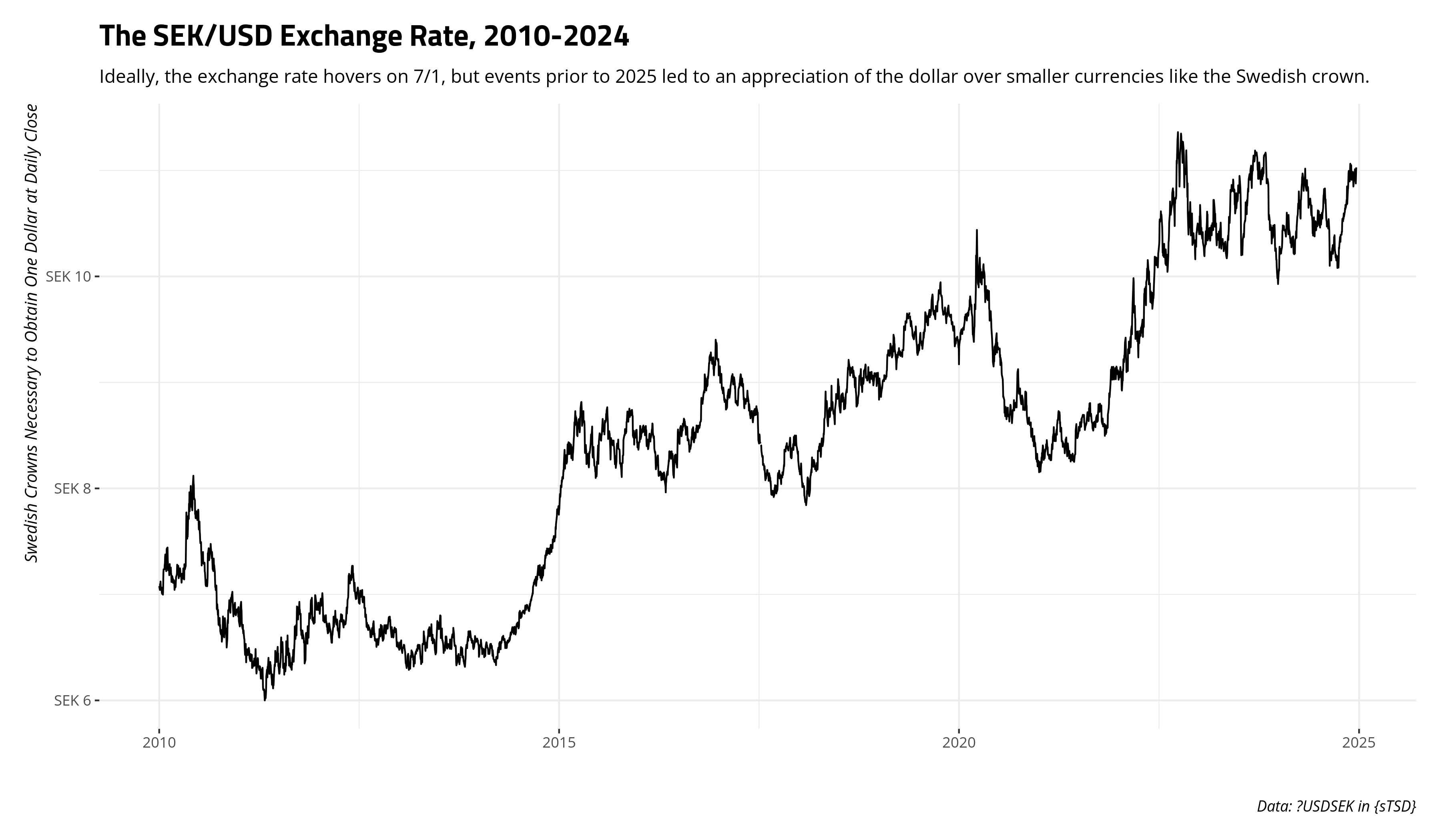
This sure looks like it would have a strong, built-in information retention mechanism. Most time series of commodities that are traded daily have a pervasive, built-in memory. We can see for ourselves with the sadf_test() function and lean on it to identify an appropriate lag structure for us.

DF4 <- sadf_test(USDSEK$close, n_sims = 500)
DF5 <- sadf_test(diff(USDSEK$close), sim_hyp = "stationary", n_sims = 500) # I'm going somewhere with this...

ur_summary(DF4)
#> ---------------------------------------------------- 
#> * Simulated (Augmented) Dickey-Fuller Test Summary * 
#> ---------------------------------------------------- 
#> Simulated test statistics are calculated on time series that are: nonstationary 
#> Length of time series: 3900. Lags: 9
#> 
#> Type 1: no drift, no trend 
#> --------------------------
#> Your tau: 1.078
#> Potential thresholds for your consideration: -2.554 (1%); -1.964 (5%); -1.557 (10%)
#> 
#> Type 2: drift, no trend
#> -----------------------
#> Your tau: -0.683
#> Potential thresholds for your consideration: -2.504 (1%); -1.802 (5%); -1.415 (10%)
#> 
#> Type 3: drift and trend
#> -----------------------
#> Your tau: -2.893
#> Potential thresholds for your consideration: -3.868 (1%); -3.368 (5%); -3.094 (10%)
#> 
#> 
#> --------------------------------------------------------------
#> * Guides to help you assess stationarity or non-stationarity * 
#> --------------------------------------------------------------
#> These thresholds are the results of 500 different simulations of a non-stationary time series matching your time series description (n = 3900, lags = 9). If your tau is more negative than one of these thresholds of interest, that is incompatible with a non-stationary time series and more compatible with a stationary time series.
#> 
#> If this is not the case, what you see is implying your time series is non-stationary.
#> 
#> Please refer to the raw output for the simulations for other means of assessment/summary.

The test statistics are compatible with a distribution of test statistics of a random walk, leading us to reasonably conclude that our times series of a currency exchange rate traded daily is non-stationary. Of course it would be.

However, it would be illustrative to get an idea of what this looks like, visually. Here, the tests included in {sTSD} allow you to evaluate your time series against a stationary or non-stationary time series. Inference in the case of the Dickey-Fuller test is traditionally made against a non-stationary time series. However, you could simulate against a stationary time series to get an idea of what the test statistics would resemble for a time series with the length and number of lags requested. That, I think, is one feature missing when your critical values are handed down from on high based on what was computationally possible or feasible 50 years ago. We know from pen-and-napkin that the first difference should be stationary, so let’s also show what the test statistics from the first-difference time series looks like compared to a distribution of test statistics from a stationary time series.

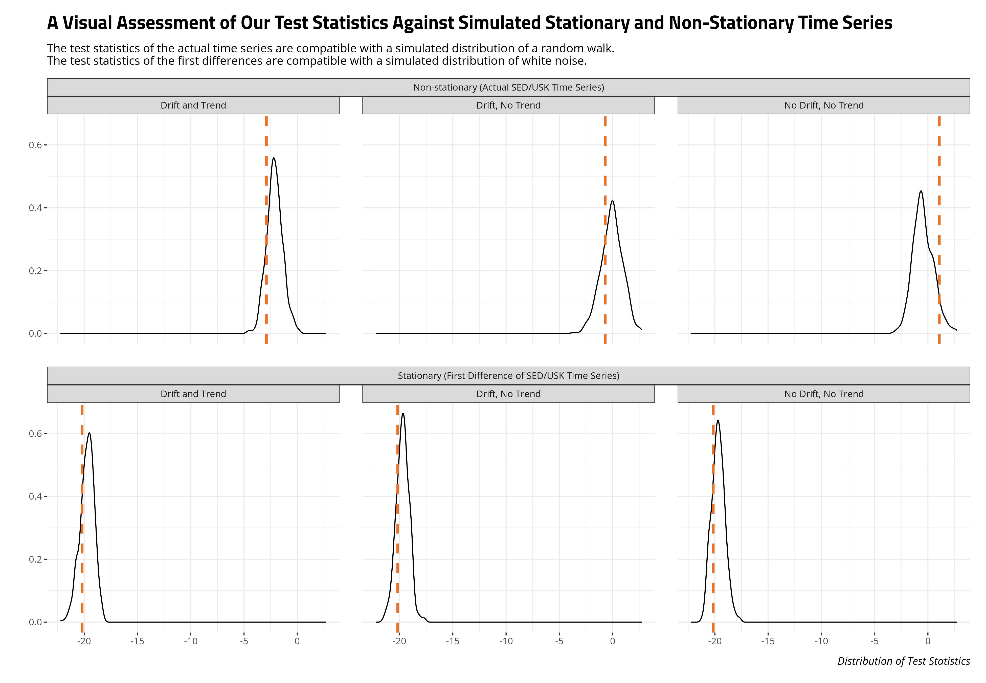
Computational abilities of the time made it impractical to simulate distributions of stationary test statistics of the Dickey-Fuller procedure when the distribution of stationary test statistics depended on the non-1 values of \(\rho\) and the length of the series. The distribution of test statistics for maximally autoregressive series were much more stable and predictable by comparison. Even though the procedure is traditionally done with the null hypothesis of non-stationary, you can assess your test statistics against simulations of a stationary time series all the same. Do what you want with the p-value under those circumstances, which is really the case for anything involving a p-value.

Conclusion

There really isn’t much to conclude here. It’s more of a quick introduction/tutorial for the MA students in our department who have to learn about unit root testing with my {sTSD} package. I never quite liked the R packages that were available in how they communicated the information of interest. Plus, it doesn’t make much sense these days to rely on old critical values generated 50 years ago for non-standard distributions like the one underpinning the (Augmented) Dickey-Fuller test. You can simulate those for yourselves. Moses can give you commandments and you just run with premise, supposedly. You can do the same here if you’d like, but simulation is much more informative.