Linear Model Diagnostics by IR Example

- Peru's Truth and Reconciliation Commission, which ran from 2001 to 2003, was tasked with investigating the human rights abuses committed in the country during its armed conflict with Sendero Luminoso. It may have further signaled to investors that Peru was serious about peace.
I’m teaching a first-year MA-level quantitative methods course at the moment for which the current topic is linear model diagnostics. The particular example that I had time and space to give them resulted in a situation where there were heteroskedastic errors, albeit with no major inferential implications whatsoever. This understandably led a student to ask if there was a case where heteroskedasticity and assorted heteroskedasticity robustness tests resulted in major inferential implications. The best answer you could give is “of course, but you wouldn’t know until you checked”. I could definitely give a U.S.-focused example that wouldn’t resonate with a European audience. However, the time and space I had before starting the class didn’t give me time to find an example that students in IR might actually understand. Even then, there aren’t many (simple) linear models you encounter in international relations. Most of the things we care about happen or don’t (and are thus better modeled through a logistic/probit regression) or have lots of moving pieces (i.e. are panel models) that are outside the bounds of the class.
There is, however, one example to offer. We should all thank Joshua Alley for beginning to curate a repository on cross-sectional OLS models around which you can teach in political science and international relations. One of those data sets is from a 2012 publication by Benjamin J. Appel and Cyanne E. Loyle in Journal of Peace Research on the economic benefits of post-conflict justice. This is an interesting paper to read with an intuitive argument and application. They argue that post-conflict states that engage in some kind of post-conflict justice initiative—like truth and reconciliation commissions or reparations—are getting a downstream benefit from it relative to states that do not do this. These states are signaling to outside investors that they are serious about peace, notwithstanding the conflict that would otherwise make them risky investments. As a result, we should expect, and the authors indeed report, that post-conflict states that engage in post-conflict justice institutions have higher levels of net foreign direct investment (FDI) inflows 10 years after a conflict ended compared to post-conflict states that do not have these institutions. Their data is rather bite-sized too: 95 observations of conflict and 10-year windows afterward for a temporal domain around 1970 to 2001.
There’s a lot to like about the argument, and certainly the data for pedagogical purposes. It’s a rare case of a simple OLS with a straightforward IR application. There’s also all sorts of interesting things happening in it that are worth exploring.
Here are the R packages we’ll be using for this post.
library(tidyverse)     # for most things
library(stevemisc)     # for helper functions
library(kableExtra)    # for tables
library(stevedata)     # for the data
library(modelsummary)  # for being awesome
library(dfadjust)      # for DF. Adj. standard errors, a la Imbens and Kolesár (2016)
library(stevethemes)   # for my themes
library(lmtest)        # for model diagnostics/summaries
library(sandwich)      # for the majority of standard error adjustments.

theme_set(theme_steve())
The Data and the Model
This simple exercise will just replicate Model 1 of what is their Table I. Here, we’re going to set up a simple model whose purpose can be phrased as follows. Appel and Loyle (2012) are proposing that scholars interested in the variation in net FDI inflows have only looked at net FDI inflows from an economic perspective. They’re missing an important political perspective (i.e. post-conflict justice institutions). Perhaps we could adequately model an economic indicator like net FDI inflows with important economic correlates, but there’s a political element that Appel and Loyle are proposing. However, to justify their political perspective, they need to control for the important economic determinants of net FDI inflows. Perhaps it’s reasonably exhaustive to model net FDI inflows as a function of gross domestic product (GDP) per capita (econ_devel), GDP (econ_size), GDP per capita growth (econ_growth, over a 10-year period), capital openness (kaopen), exchange rate volatility (xr), labor force size (lf), and life expectancy for women (lifeexp). However, there’s still an important political determinant of net FDI inflows—post-conflict justice (pcj)—even “controlling” for those things.
Let’s explore this with the EBJ data in {stevedata}, which is just a reduced form of their replication data. Their Stata code makes clear this is just a simple linear model with no adjustments reported for heteroskedasticity or “robustness”. The following code will perfectly reproduce their Model 1 in Table I. {modelsummary} will quietly format the results into a regression table.
M1 <- lm(fdi ~ pcj + econ_devel + econ_size + econ_growth + kaopen + xr + lf + lifeexp, EBJ)
| Replication | |
|---|---|
| Post-conflict Justice | 1532.608* |
| (629.400) | |
| Economic Development | −0.058 |
| (0.134) | |
| Economic Size | 0.000* |
| (0.000) | |
| Economic Growth | 0.724 |
| (21.298) | |
| Capital Openness | 132.574 |
| (208.004) | |
| Exchange Rate | −49.220* |
| (13.561) | |
| Labor Force | 14.719 |
| (25.454) | |
| Life Expectancy (Female) | 17.395 |
| (30.288) | |
| Intercept | −2011.642 |
| (2677.858) | |
| Num.Obs. | 95 |
| R2 Adj. | 0.370 |
| + p < 0.1, * p < 0.05 |
I will leave the reader to compare the results of Model 1 here to Model 1 of Table I in their paper. The basic takeaways are the same; the results are the exact same. Controlling for the economic determinants of net FDI inflows, there is a statistically significant relationship between post-conflict justice and net FDI inflows among these post-conflict states. Post-conflict states with post-conflict justice institutions have higher levels of net FDI inflows than post-conflict states without them. The estimated difference between them is ~$1532.61. If the true relationship were 0, the probability we observed what we observed would’ve happened 16 times in a thousand trials, on average.
What to Do (and Anticipate) About Non-Linearity
We teach students that one major assumption about the linear model is that the model is both linear and additive. In other words, the estimate of y (here: net FDI inflows) is an additive combination of the regressors (and an error term). The regression lines are assumed to be straight. A first cut to see if this assumption is satisfied is the fitted-residual plot. Plot the model’s fitted values on the the x-axis and the residuals on the y-axis as a scatterplot. By definition, the line of best fit through the data is flat at 0. Ideally, a LOESS smoother agrees with it.
broom::augment(M1) %>%
  ggplot(.,aes(.fitted, .resid)) +
  geom_point() +
  geom_smooth(method="loess") +
  geom_hline(yintercept = 0, linetype ='dashed')
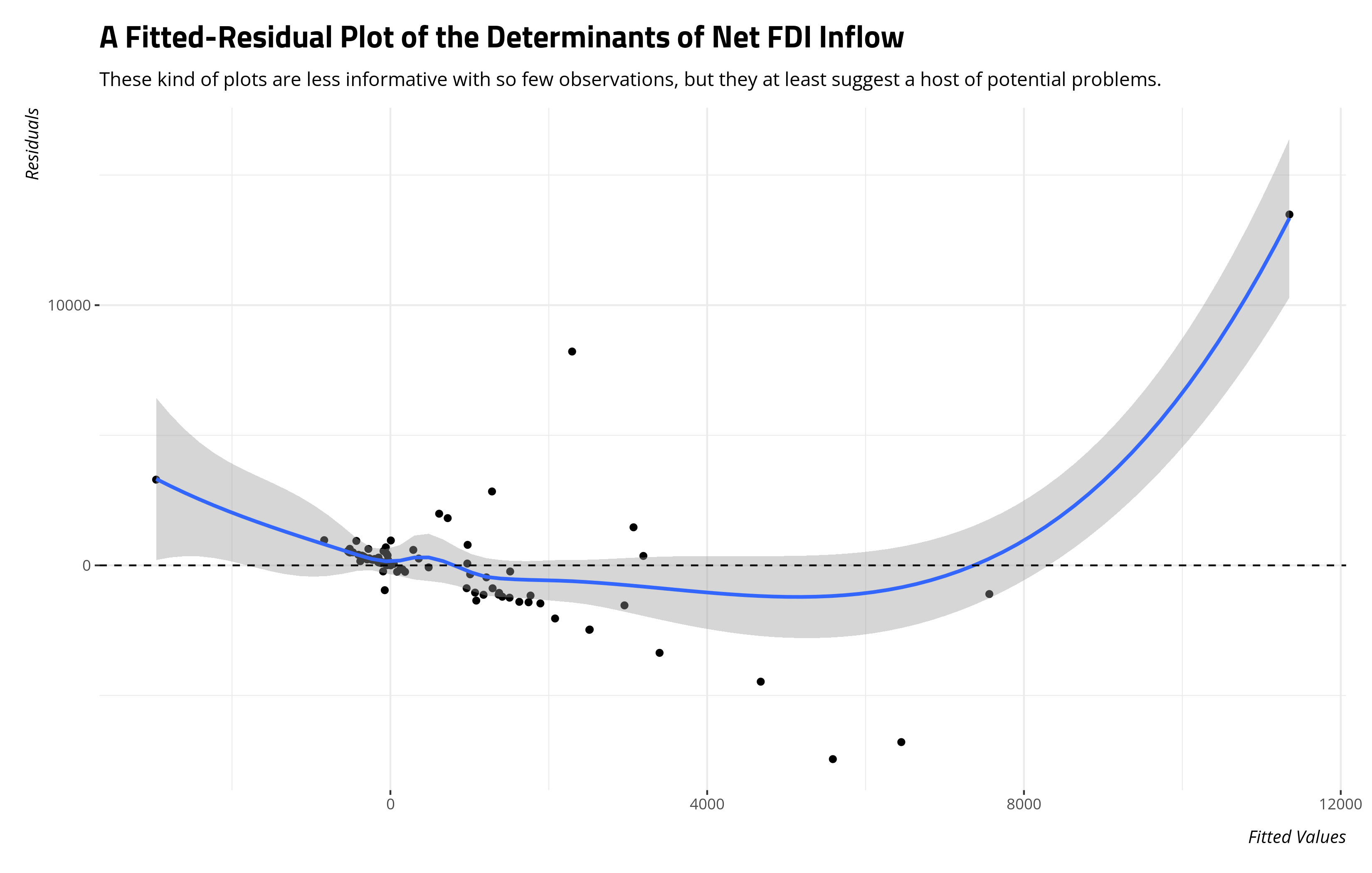
This plot has great informational value as a diagnostic (i.e. it’s also suggesting to me I have heteroskedastic errors). Here, it’s clearly telling me I have weirdness in my data that suggests non-linearity evident in the model betrays the assumption of linearity. It comes with two caveats, though. For one, a model with just 95 observations isn’t going to have a fitted-residual plot that is as easy to decipher as a plot with several hundred observations. Two, the fitted-residual plot will suggests non-linearity but won’t tell me where exactly it is.
I have a function in {stevemisc} that offers some illustrative evidence of where the non-linearity might be, along with other things that may be worth considering.1 linloess_plot(), by default, will make bivariate comparison’s of the model’s residuals with all right-hand side variables. It will overlay over it the line of best fit (0 by definition) and a smoother of your choice (default is LOESS). Where the two diverge, it suggests some kind of non-linearity. Trial and error with the function’s arguments will produce something that’s at least presentable.
linloess_plot(M1, span=1, se=F)
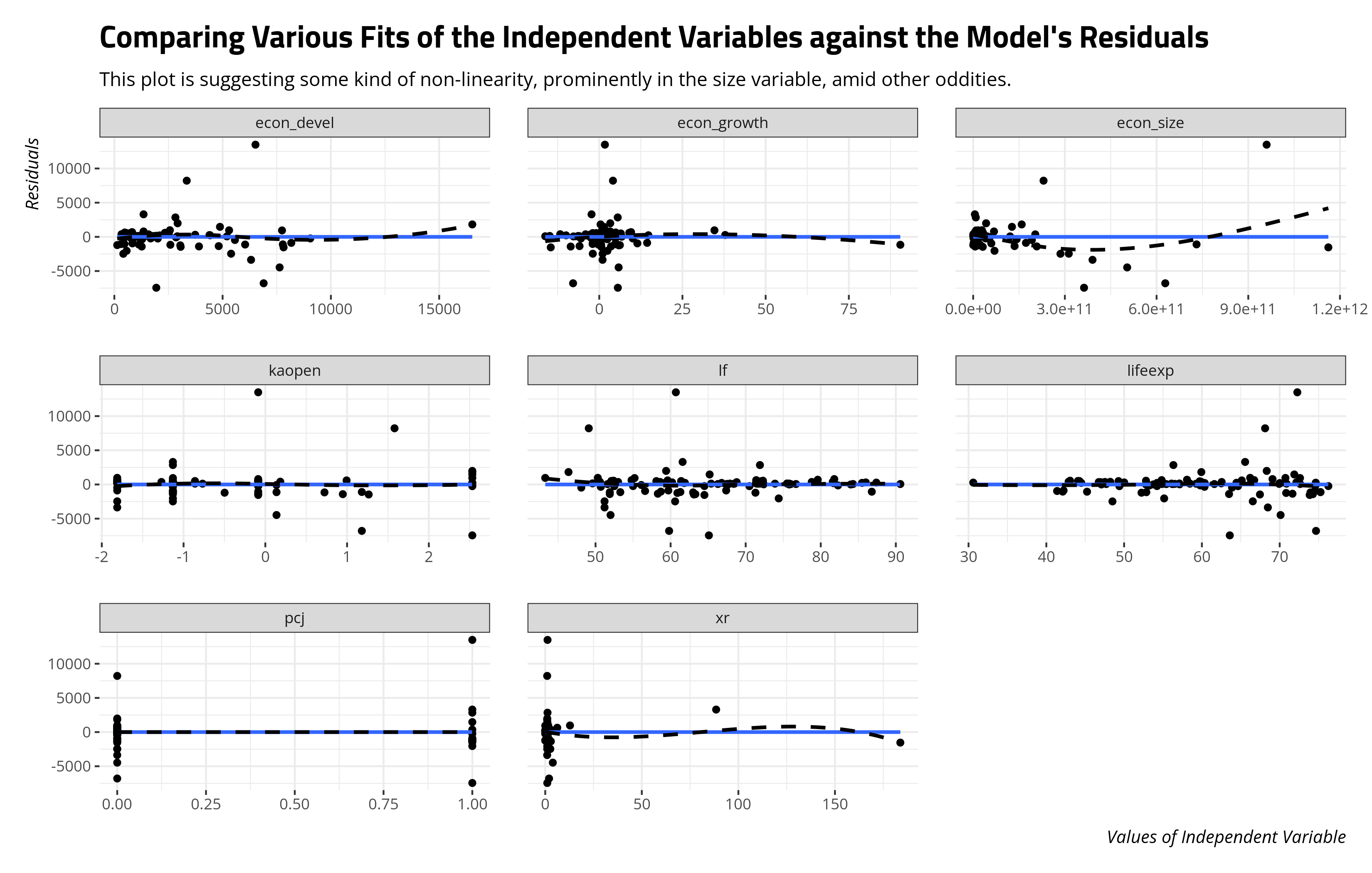
There’s a lot to unpack here (acknowledging that binary IVs will never be an issue here). Ideally, we would have more observations (i.e. the LOESS smoother is going to whine a bit for the absence of data points in certain areas), but it’s pointing to some weirdness in several variables. The exchange rate variable mostly clusters near 0, though there are a few anomalous observations that are miles from the bulk of the data. The development, growth, and size variables are all behaving weirdly. For one, it’s going to immediately stand out that these variables are on their raw scale. In other words, the economic size variable for the fourth row (for which ccode == 70 [Mexico]) is 628,418,000,000. It’s tough to say anything definitive in the absence of more information (i.e. when exactly is this GDP for Mexico and is it benchmarked to some particular dollar), it’s still very obvious this is raw dollars. Curvilinearity is evident in this, but that curvilinearity may not have emerged had this been log-transformed.
Indeed, a lot of what is shown here could’ve been anticipated by looking at the data first.
EBJ %>%
  select(fdi:lifeexp, -pcj) %>%
  gather(var, val) %>%
  ggplot(.,aes(val)) + geom_density() +
  facet_wrap(~var, scales='free')
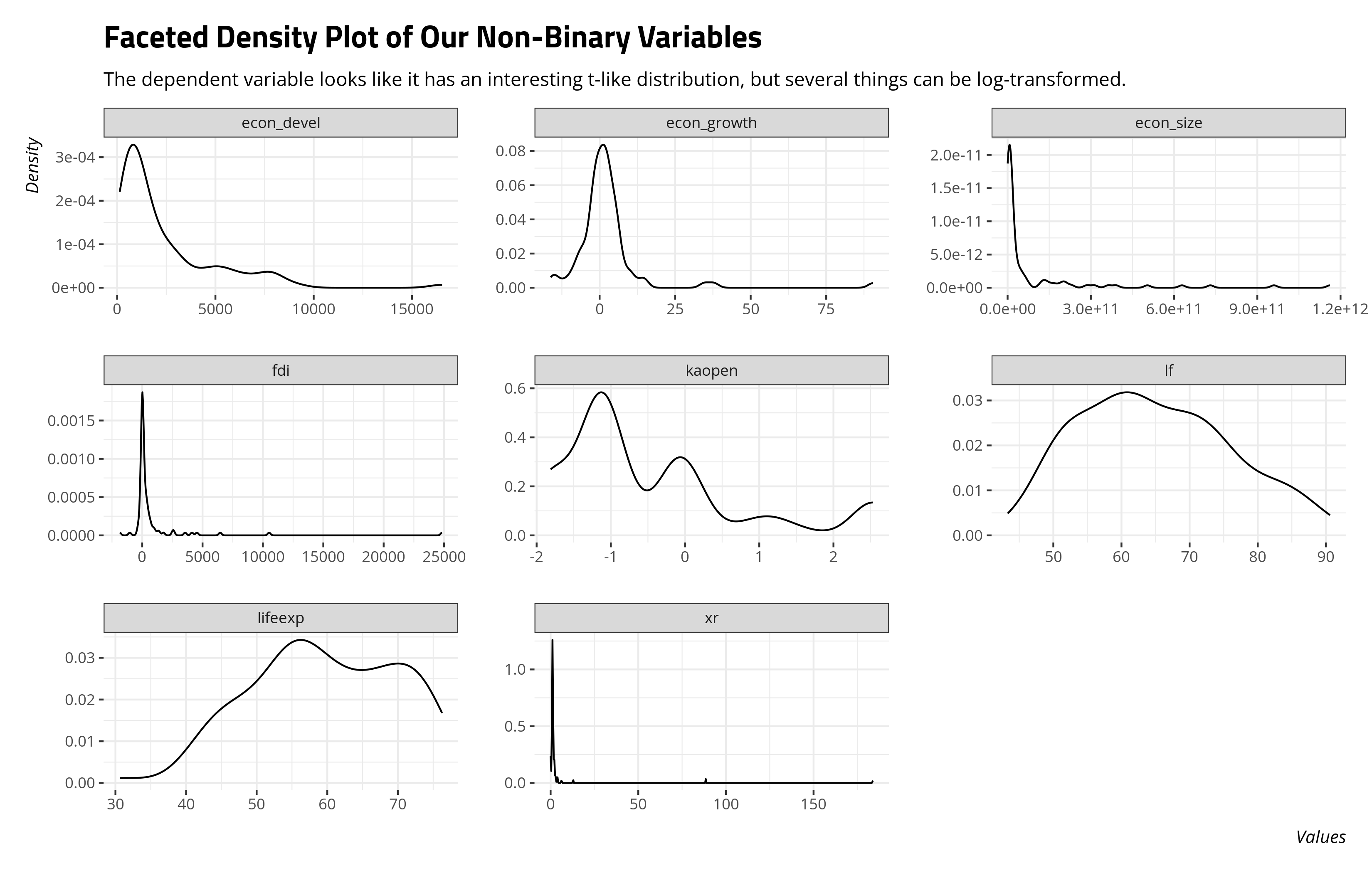
There are some obvious design choices you could make from this. We should 100% log-transform the GDP and GDP per capita variable. One is obvious, but has a caveat worth belaboring for real variables with 0s. Practitioners would +1-and-log that exchange rate variable and perhaps we can do that here without controversy. Some are less obvious. The economic growth variable and FDI variable both have negative values, so logarithmic transformations without an additive constant are not available to us. The economic growth variable is still mostly fine as a distribution, but has two anomalous values far to the right. The FDI variable has a very interesting distribution. It’s almost like a Student’s t-distribution with three or fewer degrees of freedom. I have an idea of what I’d like to do with this variable for pedagogical purposes, but I’ll save that for another post.
For now, let’s do this. Let’s log-transform the development and size variables, +1-and-log the exchange rate variable, and just wave our hands at the economic growth variable and dependent variable. If the lin-LOESS plot I introduced above is correct, it’s suggesting a square term effect of economic size that we should also model.
EBJ %>%
  log_at(c("econ_devel", "econ_size")) %>%
  mutate(ln_xr = log(xr + 1)) -> EBJ

M2 <- lm(fdi ~ pcj + ln_econ_devel + ln_econ_size +
           I(ln_econ_size^2) + econ_growth + kaopen + ln_xr + lf + lifeexp, EBJ)
| Replication | With Transformations | |
|---|---|---|
| Post-conflict Justice | 1532.608* | 1525.326* |
| (629.400) | (714.274) | |
| (Raw|Logged) Economic Development | −0.058 | 237.485 |
| (0.134) | (534.838) | |
| (Raw|Logged) Economic Size | 0.000* | −8011.586* |
| (0.000) | (3036.325) | |
| (Raw|Logged) Economic Size^2 | 179.995* | |
| (63.760) | ||
| Economic Growth | 0.724 | 0.903 |
| (21.298) | (23.958) | |
| Capital Openness | 132.574 | 104.810 |
| (208.004) | (242.793) | |
| (Raw|Logged) Exchange Rate | −49.220* | −527.487 |
| (13.561) | (400.773) | |
| Labor Force | 14.719 | 26.098 |
| (25.454) | (29.833) | |
| Life Expectancy (Female) | 17.395 | 11.338 |
| (30.288) | (42.936) | |
| Intercept | −2011.642 | 85152.614* |
| (2677.858) | (36439.112) | |
| Num.Obs. | 95 | 95 |
| R2 Adj. | 0.370 | 0.207 |
| + p < 0.1, * p < 0.05 |
The results here suggest that there was non-linearity evident in the original data, and that it’s just not a curvilinear relationship between economic size and net FDI inflows. There’s proportionality as well, some of which could’ve been anticipated. The GDP (“size”) and GDP per capita (“development”) variables are the largest nominal value possible (raw dollars to the dollar). In most applications, those would be log-transformed. The exchange rate variable could also be reasonably +1 and logged as well. Perhaps assorted other transformations in light of other peculiarities (e.g. the growth variable and the dependent variable itself) may have different implications, but even doing these transformations are sufficient to find a strong curvilinear effect of economic size and to find no discernible (proportional) effect of the exchange rate variable.
What to Do About Non-Constant Error Variance (Heteroskedasticity)
The fitted-residual plot will often give you a pretty good indication about non-constant error variance (heteroskedasticity) if you have enough observations. It’s a little harder to parse with the number of observations we have. No matter, we have a formal test diagnostic—the Breusch-Pagan test—for heteroskedasticity in the regression model. The test itself analyzes patterns/associations in the residuals as a function of the regressors, returning a test statistic (with a p-value) based on the extent of associations it sees. High enough test statistic with some p-value low enough (for whatever evidentiary threshold floats your boat) suggests heteroskedastic errors. I’m fairly sure we’re going to see that here in both our models.
bptest(M1)
#>
#> 	studentized Breusch-Pagan test
#>
#> data:  M1
#> BP = 50.535, df = 8, p-value = 3.225e-08
bptest(M2)
#>
#> 	studentized Breusch-Pagan test
#>
#> data:  M2
#> BP = 24.48, df = 9, p-value = 0.003603
I am not terribly surprised, especially since we did not touch the dependent variable (which is often, but certainly not always, the culprit in these situations). Here’s where we reiterate that the problem of heteroskedasticity is less about the line and more about the uncertainty around the line. That uncertainty is suspect, which has ramifications for those important tests you care about (i.e. tests of statistically significant associations). Thus, you need to do something to convince me that any inferential takeaways you’d like to report are not a function of this violation of the linear model with its OLS estimator.
You have options, and I’ll level with you that I think the bulk of these reduce to throwing rocks at your model to see how sensitive the inferences you’d like to report are. So, let’s go over them and start with the replication model reported by Appel and Loyle (2012) in their first model in Table I. If you were learning this material by reference to a by-the-books statistics textbook, their recommendation is weighted least squares (WLS) in this situation. Weighted least squares takes the offending model, extracts its residuals and fitted values, regresses the absolute value of the residuals on the fitted values in the original model. It then extracts those second fitted values, squares them, and divides 1 over them. Those are then supplied as weights to the offending linear model once more for re-estimation.
But wait, there’s more. If you were learning statistics by reference to an econometrics textbook, it might balk at the very notion of doing this. Their rationale might be one or both of two things. First, weighted least squares makes an assumption about the true nature of the error variance that might otherwise be unknowable. Second, if the implication of heteroskedasticity is that the lines are fine and the errors are wrong, it’s a lament that the weighted least squares approach is almost guaranteed to re-draw lines to equalize the variance in errors. If the lines are fine and the errors are wrong, the errors of the offending model can be recalibrated based on information from the variance-covariance matrix to adjust for this. This would make the standard errors “robust.”
Here, you have several options for so-called “heteroskedasticity consistent (HC)” or “robust” standard errors. Sometimes, it seems like you have too many options. The “default” (if you will) was introduced by White (1980) as an extension of earlier work by Eicker (1963) and Huber (1967). Sometimes known as “Huber-White” standard errors, or HC0 in formula syntax, this approach adjusts the model-based standard errors using the empirical variability of the model residuals. But wait, there’s even more. There are three competing options for these heteroskedasticity-consistent standard errors: HC1, HC2, and HC3, all introduced by MacKinnon and White (1985). With a large enough sample, all three don’t differ too much from each other (as far as I understand it). I’ll focus on two of the three, though. The first is HC1, which is what incidentally what Stata would use for default if you were to ask for “robust” standard errors.2 The second is HC3, which is the suggested default in the {sandwich} package we’ll be using to calculate these things. For fun, we can also provide so-called Bell-McCaffrey degrees-of-freedom adjusted (DF. Adj.) robust standard errors following the recommendations of Imbens and Kolesár (2016).
And yes, there’s even more than that. If I were presented this hypothetical situation with 95 observations and all the computing power I could ever want, I would 100% bootstrap this. You have plenty of options here. The simple bootstrap resamples, with replacement, from the data to create some number of desired replicates against which the model is re-estimated. Given enough replicates, the mean of the coefficients converges on the original coefficient but the standard deviation of the coefficient from those replicates is the new standard error. You judge statistical significance from that. There are several other bootstrapping approaches, but here’s just two more. The first is a bootstrapped model from the residuals. Rather than case resampling (with replacement), this approach takes the residuals from the offending model, resamples those with replacement, and adds the residuals to the outcome variable as new synthetic values. The regressors themselves are fixed and unchnaged, but the outcome variable is then subject to resampling of a kind. A spiritually similar approach, the so-called “wild” bootstrap, multiplies the residuals by response variable once they have been multiplied by a random variable. By default, this is a Rademacher distribution. Truthfully, if you are tempted to use the residual bootstrap, you should probably use the wild bootstrap instead.
You could do all this mostly from the vcov* family of functions in the {sandwich} package, combined with coeftest() from {lmtest}. The reproducible seed is for funsies since there’s bootstrap resampling happening here as well. We’ll go with 500 replicates (which is what the R argument is doing).
set.seed(8675309)
summary(M1)
wls(M1) # from {stevemisc}
coeftest(M1,  vcovHC(M1,type='HC0'))
coeftest(M1,  vcovHC(M1,type='HC1'))
coeftest(M1,  vcovHC(M1,type='HC3'))
dfadjustSE(M1) # from {dfadjust}
coeftest(M1,  vcovBS(M1, R = 500))
coeftest(M1,  vcovBS(M1, type='residual', R = 500))
coeftest(M1,  vcovBS(M1, type='wild', R = 500))
A better approach is to have {modelsummary} do all this for you, which is happening under the hood here.
| M1 | WLS | HC0 | HC1 | HC3 | DF. Adj. | Bootstrap | Resid. Boot. | Wild Boot. | |
|---|---|---|---|---|---|---|---|---|---|
| Post-conflict Justice | 1532.608* | 532.046 | 1532.608 | 1532.608 | 1532.608 | 1532.608 | 1532.608 | 1532.608* | 1532.608 |
| (629.400) | (1371.693) | (927.378) | (974.696) | (1371.693) | (1116.830) | (930.624) | (555.819) | (952.559) | |
| Economic Development | −0.058 | 0.056 | −0.058 | −0.058 | −0.058 | −0.058 | −0.058 | −0.058 | −0.058 |
| (0.134) | (0.224) | (0.143) | (0.150) | (0.224) | (0.175) | (0.210) | (0.128) | (0.132) | |
| Economic Size | 0.000* | 0.000 | 0.000+ | 0.000+ | 0.000 | 0.000 | 0.000+ | 0.000* | 0.000+ |
| (0.000) | (0.000) | (0.000) | (0.000) | (0.000) | (0.000) | (0.000) | (0.000) | (0.000) | |
| Economic Growth | 0.724 | 1.695 | 0.724 | 0.724 | 0.724 | 0.724 | 0.724 | 0.724 | 0.724 |
| (21.298) | (24.239) | (10.858) | (11.412) | (24.239) | (15.643) | (20.781) | (20.893) | (11.128) | |
| Capital Openness | 132.574 | 48.862 | 132.574 | 132.574 | 132.574 | 132.574 | 132.574 | 132.574 | 132.574 |
| (208.004) | (296.297) | (246.782) | (259.374) | (296.297) | (269.078) | (275.786) | (211.499) | (248.941) | |
| Exchange Rate | −49.220* | 5.207 | −49.220+ | −49.220 | −49.220 | −49.220 | −49.220 | −49.220* | −49.220+ |
| (13.561) | (59.095) | (29.017) | (30.497) | (59.095) | (38.458) | (88.112) | (11.189) | (28.015) | |
| Labor Force | 14.719 | 4.360 | 14.719 | 14.719 | 14.719 | 14.719 | 14.719 | 14.719 | 14.719 |
| (25.454) | (21.943) | (17.191) | (18.069) | (21.943) | (19.106) | (19.928) | (25.090) | (17.760) | |
| Life Expectancy (Female) | 17.395 | 2.913 | 17.395 | 17.395 | 17.395 | 17.395 | 17.395 | 17.395 | 17.395 |
| (30.288) | (26.121) | (16.125) | (16.948) | (26.121) | (19.815) | (24.037) | (30.291) | (15.941) | |
| Intercept | −2011.642 | −402.067 | −2011.642 | −2011.642 | −2011.642 | −2011.642 | −2011.642 | −2011.642 | −2011.642 |
| (2677.858) | (2100.212) | (1517.895) | (1595.344) | (2100.212) | (1747.984) | (1927.093) | (2686.032) | (1573.992) | |
| Num.Obs. | 95 | 95 | 95 | 95 | 95 | 95 | 95 | 95 | 95 |
| R2 Adj. | 0.370 | 0.241 | 0.370 | 0.370 | 0.370 | 0.370 | 0.370 | 0.370 | 0.370 |
| + p < 0.1, * p < 0.05 |
There’s a lot happening here, and we should be initially skeptical of the model with such an evident problem of skew in the economic size and development variables. No matter, this approach suggests what approach you employ for acknowledging and dealing with the heteroskedasticity in your model has important implications for the statistical (in)significance you may like to report. The post-conflict justice variable is significant only in the replication model and the residual bootstrapping approach. The economic size variable is insignificant in the WLS, HC3, and DF. Adj. approach. The exchange rate variable is significant only in the original model, the model with Huber-White standard errors (HC0), and two of the three bootstrapping approaches. We could note, though, it is a judgment call at the .10 level and we should be humble about making binary classifications of “significant” versus “not significant” based on this tradition. But, make of that what you will.
We can do the same thing to the second model, which offers logarithmic transformations of economic development, economic size, and the exchange rate variable (in addition to the square term of economic size).
| M2 | WLS | HC0 | HC1 | HC3 | DF. Adj. | Bootstrap | Resid. Boot. | Wild Boot. | |
|---|---|---|---|---|---|---|---|---|---|
| Post-conflict Justice | 1525.326* | 480.933 | 1525.326 | 1525.326 | 1525.326 | 1525.326 | 1525.326 | 1525.326* | 1525.326 |
| (714.274) | (1389.818) | (1135.250) | (1200.173) | (1389.818) | (1255.379) | (1198.794) | (632.009) | (1118.279) | |
| Logged Economic Development | 237.485 | −199.705 | 237.485 | 237.485 | 237.485 | 237.485 | 237.485 | 237.485 | 237.485 |
| (534.838) | (520.918) | (432.055) | (456.764) | (520.918) | (472.807) | (509.681) | (491.713) | (448.304) | |
| Logged Economic Size | −8011.586* | −1501.301 | −8011.586 | −8011.586 | −8011.586 | −8011.586 | −8011.586 | −8011.586* | −8011.586 |
| (3036.325) | (6955.913) | (5589.389) | (5909.037) | (6955.913) | (6228.081) | (5975.243) | (3107.540) | (5466.750) | |
| Logged Economic Size^2 | 179.995* | 34.710 | 179.995 | 179.995 | 179.995 | 179.995 | 179.995 | 179.995* | 179.995 |
| (63.760) | (153.167) | (123.255) | (130.304) | (153.167) | (137.249) | (131.544) | (65.556) | (120.363) | |
| Economic Growth | 0.903 | 5.926 | 0.903 | 0.903 | 0.903 | 0.903 | 0.903 | 0.903 | 0.903 |
| (23.958) | (21.520) | (9.468) | (10.009) | (21.520) | (13.772) | (16.901) | (21.151) | (9.405) | |
| Capital Openness | 104.810 | 146.835 | 104.810 | 104.810 | 104.810 | 104.810 | 104.810 | 104.810 | 104.810 |
| (242.793) | (309.297) | (262.045) | (277.030) | (309.297) | (284.372) | (289.418) | (227.233) | (273.986) | |
| Logged Exchange Rate | −527.487 | −23.880 | −527.487 | −527.487 | −527.487 | −527.487 | −527.487 | −527.487 | −527.487 |
| (400.773) | (579.782) | (412.935) | (436.550) | (579.782) | (484.176) | (479.507) | (402.422) | (402.086) | |
| Labor Force | 26.098 | 14.134 | 26.098 | 26.098 | 26.098 | 26.098 | 26.098 | 26.098 | 26.098 |
| (29.833) | (26.041) | (21.609) | (22.845) | (26.041) | (23.664) | (25.434) | (25.869) | (21.805) | |
| Life Expectancy (Female) | 11.338 | 22.923 | 11.338 | 11.338 | 11.338 | 11.338 | 11.338 | 11.338 | 11.338 |
| (42.936) | (25.646) | (20.351) | (21.515) | (25.646) | (22.537) | (27.335) | (38.024) | (20.538) | |
| Intercept | 85152.614* | 15469.080 | 85152.614 | 85152.614 | 85152.614 | 85152.614 | 85152.614 | 85152.614* | 85152.614 |
| (36439.112) | (76889.954) | (61649.423) | (65175.048) | (76889.954) | (68759.859) | (66377.553) | (37504.039) | (60299.811) | |
| Num.Obs. | 95 | 95 | 95 | 95 | 95 | 95 | 95 | 95 | 95 |
| R2 Adj. | 0.207 | 0.726 | 0.207 | 0.207 | 0.207 | 0.207 | 0.207 | 0.207 | 0.207 |
| + p < 0.1, * p < 0.05 |
A similar story will still emerge. What statistical significance you’d like to report is sensitive to the heteroskedasticity in the original model and how you elected to acknowledge it and deal with it. Post-conflict justice and the economic size variables are significant in only one of the adjustments (incidentally: the residual bootstrap). It’s at least a little amusing that a model that better incorporates the proportionality of key right-hand side predictors, and makes a reasoned post-estimation design choice to re-estimate with a square term, results in new models for which “robustness” often suggests no discernible effects at all. But again, make of that what you will.
Conclusion
The point here isn’t to chastise past scholarship or deride the work done by others. It’s also not to litigate whether there’s value to post-conflict justice institutions. Sometimes there’s value—normative value—in making amends for past wrongs and broadcasting what exactly those wrongs were irregarding whether there’s a downstream benefit in which investors part with their money and send it to you. The point is instead that some anticipatory diagnostics and rudimentary model diagnostics can materially change the inferences you’d like to report.
Make reasoned design choices about what you can anticipate about the distribution of the inputs into your model. That might indicate in advance the kind of non-linearity the fitted-residual plot will suggest from your basic linear model. It may suggest proportional/magnitude changes that are not linear on its raw scale. Making reasoned choices about what to do with these before running the model may change the inferences you’d like to report. Choosing post-modeling re-estimation techniques based on model diagnostics may lead to re-estimations that further change the inferences you’d like to report.
It is also the case that heteroskedasticity, and how you elect to deal with it, can matter a great deal to your test statistics. The presence of heteroskedasticity means the important test statistics you care about are suspect. If those test statistics are that sensitive to a model that violates an important assumption, and to a particular approach that deals with that particular violation, it may be worth noting the results you’d like to emphasize are potentially a function of these choices.
-
I will concede that the
residualPlots()function in{car}is far, far better for the task at hand. However, I want to avoid function clashes with{tidyverse}as much as I can. ↩ -
I’ll be honest that I have no idea how how this became the default standard error correction in Stata. I wish I did. I just know that it was when I was using Stata (and might still be, for all I know). ↩
Disqus is great for comments/feedback but I had no idea it came with these gaudy ads.