(Quasi)-automating the Inclusion of Random Effects in R's Stargazer Package
- Consider Reading This Post Instead ⤵️
- You can read this if you'd like, but I recently wrote about a better solution for the motivating question that probably brought you here.
- A Better Way to Include Random Effects for Mixed Effects Models in a Stargazer Table
There's a better way to include effects about random parameters from a mixed effects model in a table made by R's stargazer package. 15 May 2020
stargazer is a godsend for those of us who look for seamless ways to manage the execution and presentation of our statistical analyses. LaTeX, for all its strengths, inconveniences users who need to manually create tables. Doing this for peer-reviewed scholarship can be a perilous process, greatly increasing the probability of human error in the presentation of the results. The stargazer package, as all useful packages do, automates that and makes it the job of R to render the regression table. It also handles lmer output, which is fantastic for those of us who estimate mixed effects models as models of choice.
However, one limitation of the stargazer package is that it ultimately processes lmer output no different than it would handle a standard linear model or generalized linear model. It reports only the fixed effects of the model, even though the whole point of mixed effects models is that they contain important quantities of interest known as random effects. When these models are estimated, these parameters should be communicated in the regression table as well. In most standard models, following discussion in the likes of Andrew Gelman and Jennifer Hill’s book, these quantities of interest are typically just the number of unique observations in the random effect (i.e. “the number of groups”) and the standard deviation of the random effect. This second quantity of interest, which is standard output from an lmer model, communicates the variation in the group intercepts left unexplained after the fixed effects of the model are estimated.
Normally, the analyst can just manually insert these into the stargazer output. However, with some effort, this can be automated as well. This assumes that LaTeX is the output the researcher wants and the researcher is proficient in LaTeX tags.
I illustrate this process below using the cake data that comes with the lme4 package. First, let’s understand the data. The lme4 reference manual describes the cake data set as follows.
Data on the breakage angle of chocolate cakes made with three different recipes and baked at six different temperatures. This is a split-plot design with the recipes being whole-units at the different temperatures being applied to sub-units (within replicates). The experimental notes suggest that the replicate numbering represents temporal ordering.
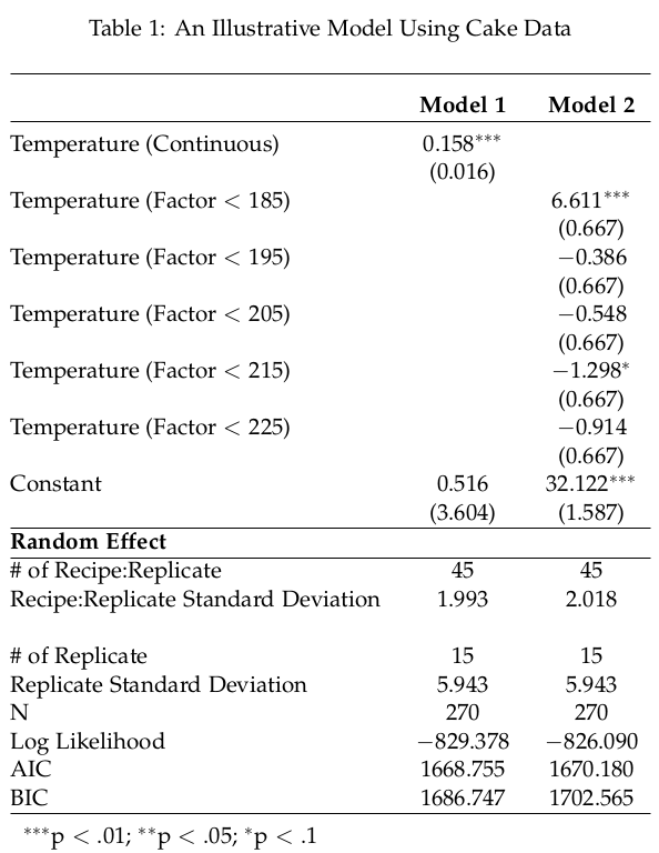
The substance of the experiment is beyond the expertise of the political scientist, though I heard “cake” and “data” and that’s all I needed to hear. We’ll be estimating the outcome variable (angle) as a function of the temperature at which it was cooked. The first model will be the temperature as a continuous variable. The second model will break the temperature variable into ordered factors, leaving the (< 175) category as the baseline comparison.
We’ll also estimate two random effects for each model. The first random effect will be each unique combination of the replicate variable (a factor variable with 15 different values) and the recipe variable (which was three, described earlier). All told, there are 45 different values in the first random effect (i.e. 15*3 = 45). The second random effect will be just the replicate variable.
Let’s get started in R, loading the two required packages for this exercise and the data to be used.
library(lme4)
library(stargazer)
data(cake)
Let’s also load in a manual function that will allow us to insert new rows at various points in a data frame.
insertrow <- function(existingDF, newrow, r) {
 existingDF[seq(r+1,nrow(existingDF)+1),] <- existingDF[seq(r,nrow(existingDF)),]
 existingDF[r,] <- newrow
 existingDF
}
This is a simple function and its use will be seen in clearer detail soon.
Next, let’s estimate and get summaries of our two models.
summary(M1 <- lmer(angle ~ temp + (1 | replicate) + (1|recipe:replicate), cake, REML= FALSE))

summary(M2 <- lmer(angle ~ factor(temperature) + (1 | replicate) + (1|recipe:replicate), cake, REML= FALSE))
Next, let’s use the stargazer command to create the broad template for our table. I keep it simple in this stargazer call, just eliminating the dependent variable label and providing labels for the covariates. Do consult Jake Russ’ quite handy cheatsheet for stargazer if you want to know more about how to master this package.
Tables <- stargazer(M1, M2, style="ajps", title="An Illustrative Model Using Cake Data", dep.var.labels.include = FALSE,
 covariate.labels=c( "Temperature (Continuous)", "Temperature (Factor $<$ 185)", "Temperature (Factor $<$ 195)", "Temperature (Factor $<$ 205)", "Temperature (Factor $<$ 215)", "Temperature (Factor $<$ 225)")
)
Now, let’s convert this new object that we titled Tables as a data.frame and coerce the one vector in it (also called Tables) into a character.
Tables <- as.data.frame(Tables)
Tables$Tables <- as.character(Tables$Tables)
Tables
Manually spit out the object (i.e. the Tables call) to see where you want to insert the information about the random effects. This is typically done above the model fit information and after the last row of standard errors for the fixed effects. In this case, I see I’m starting at row 25. Make a note of it as follows.
# Find where you want to put in the random effect. In our case, this is right after the last fixed effect. Line: 25.

r <- 25
This will be placeholder information and it’s useful to keep a note of it. Next, create some standard rows you’ll want to add. You can do this in R.
randomeffect <- "{\\bf Random Effect} & & \\\\"
hline <- "\\hline"
newline <- "\\\\"
Recall that characters in R that include backslashes should be preceded by an additional backslash. This is why you see double the normal backslashes for LaTeX tags.
Now, starting at row 25 in that Tables object, let’s add a horizontal line, a row partitioning the random effect information to follow, and another horizontal line.
Tables <- insertrow(Tables, hline, r)
Tables <- insertrow(Tables,randomeffect,r+1)
Tables <- insertrow(Tables,hline,r+2)
Notice this is where we start using the insertrow function we outlined earlier. This function identifies a table data.frame (here: Tables). Then, it inserts a row of whatever you want (e.g. hline, randomeffect) at starting point r (which we specified earlier as row 25). It pushes everything else from the row number identified down one spot.
The next step is to know the order of your random effect groupings. Generally, I think “last comes first” is how lme4 stores lmer output. The first random effect specified in the lmer call is the last random effect stored in the lmer output. Therefore, the recipe:replicate combination is the first random effect and the replicate random effect comes second. Let’s get the number of unique values in each of the groupings.
num.recipe.replicate <- sapply(ranef(M1),nrow)[1]
num.replicate <- sapply(ranef(M1),nrow)[2]
If you were to just run those commands without storing the output, you’d see the integers are 45 and 15 respectively. They don’t vary (in our case) from the first model to the second. If they do, grab them from the second model and store them as another output in your R environment.
Next, let’s get the standard deviation of the random effect, which communicates the amount of variation among the different groupings left unexplained after the estimation of the fixed effects in the model. Look careful at how this information can be extracted from lmer output.
stddev.M1.recipe.replicate <- attributes(VarCorr(M1)$"recipe:replicate")$stddev

stddev.M1.replicate <- attributes(VarCorr(M1)$replicate)$stddev

stddev.M2.recipe.replicate <- attributes(VarCorr(M2)$"recipe:replicate")$stddev

stddev.M2.replicate <- attributes(VarCorr(M2)$replicate)$stddev
Now, we’re going to use the paste function to create a free-floating character row. Notice that anything in quotes will be passed as a character into the assigned output. You can “pause” this by closing a quote, adding a comma, and assigning an R object. Follow it with a comma and resume with characters in quotes.
Some important notes about what’s happening here. Since we have just two models we’re including, we need just two ampersands to separate the quantities of Model 1 from Model 2. Further, since this is LaTeX output we’re wanting, make sure you close with four backslashes. Observe.
number.of.recipe.replicate <- paste("\\# of Recipe:Replicate & ", num.recipe.replicate, "&", num.recipe.replicate, "\\\\")

stddev.recipe.replicate <- paste("Recipe:Replicate Standard Deviation & ", round(stddev.M1.recipe.replicate, 3), "&", round(stddev.M2.recipe.replicate, 3), "\\\\")
Let’s see what this did.
> number.of.recipe.replicate
[1] "\\# of Recipe:Replicate & 45 & 45 \\\\"

> stddev.recipe.replicate
[1] "Recipe:Replicate Standard Deviation & 1.993 & 2.018 \\\\"
This is glorified LaTeX output, stored as a character in R.
Now, let’s do the same for the information about the random effects for the second model.
number.of.replicate <-paste("\\# of Replicate & ", num.replicate, "&", num.replicate, "\\\\")

stddev.replicate <- paste("Replicate Standard Deviation & ", round(stddev.M1.replicate, 3), "&", round(stddev.M2.replicate, 3), "\\\\")
Here’s the fun part. Let’s add them all together now with our insertrow function.
Tables <- insertrow(Tables,number.of.recipe.replicate,r+3)
Tables <- insertrow(Tables,stddev.recipe.replicate,r+4)
Tables <- insertrow(Tables,newline,r+5)
Tables <- insertrow(Tables,number.of.replicate,r+6)
Tables <- insertrow(Tables,stddev.replicate,r+7)
Save as if it were a table, but give it a .tex extension. Use these options to make sure you don’t get row names, column names, or quotes around the characters.
write.table(Tables,file="tables.tex",sep="",row.names= FALSE,na="", quote = FALSE, col.names = FALSE)Assuming you have a LaTeX/R workflow setup where you could immediately render your LaTeX document with your new table, you’ll get output like this.
- LaTeX table made and modified in R.
If you’re proficient with LaTeX, this will look at lot more intuitive. It is a convoluted way to automate this process, though the payoff comes later in the analysis process when different tweaks are made and time is saved from having to manually re-enter random effects into the regression table. It would be fantastic if the stargazer package could do this automatically. Until then, here is a way to quasi-automate the inclusion of random effects into stargazer output.
Code for this exercise will be made available at my Github page.
Disqus is great for comments/feedback but I had no idea it came with these gaudy ads.