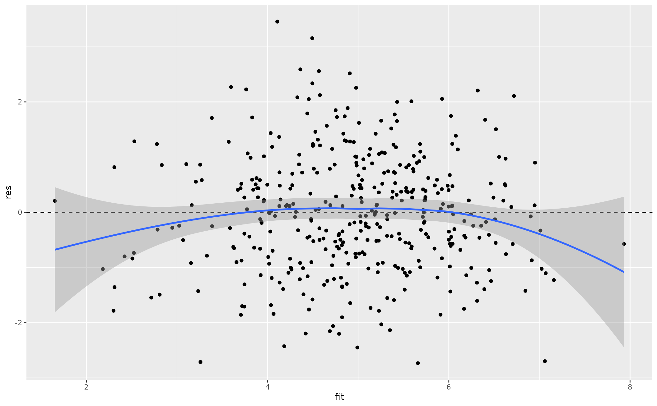
fr_plot() provides a visual diagnostic of the linearity
assumption and the homoskedasticity assumption of the linear model. Provided
an OLS model fit by lm() in
base R, the function extracts the fitted values and the residuals of the
model. Then, it creates a scatterplot of them. By definition, the line of
best fit through this scatterplot is flat at 0. A LOESS smoother, drawn over
the top of this scatterplot, provides a visual assessment of whether this
relationship that is true by definition is a reasonable summary of the
relationship between the fitted values and the residuals. The plot allows
for a visual assessment of the variation of the residuals across the range
of the fitted values as well. The function may be used
for diagnostic purposes.
Value
fr_plot() returns a scatterplot of the fitted values and
residuals of a linear model, as a ggplot2 object. The relationship
between the fitted values and the residuals is flat at 0 by definition. A
LOESS smoother offers another route to an interpretation of how one might
describe this relationship.
Details
The user can always add ggplot2 elements on top of this for greater legibility/clarity.
This function is targeted toward students I teach as a kind of convenience function when teaching linear models.
This function right now will issue a stop if the model provided is not of type
"lm" generated by the lm() function in base R.